Author's accepted manuscript

This page is the author's accepted manuscript (AAM) of a paper in preparation for Engineering Structures (consolidated from the earlier MSSP26-1185 submission that was rejected with invitation to resubmit as a new paper). Status: drafting; target submission 2026-06-15. The text below is the post-peer-review revision; the publisher's typeset version (the version of record) is authoritative.

Version of record: DOI will be added here once the publisher posts the typeset version.

Shared under CC BY-NC-ND 4.0, in accordance with the publisher's author-sharing policy.

Summary¶

Full title¶

Physics-Informed Environmental Compensation for Vibration-Based Scour Detection on Offshore Wind Turbine Foundations: State-Function Theory, Cointegration Equivalence, Four-Method Benchmark, and Thirty-Two-Month Field Demonstration.

One-sentence headline¶

A state-function decomposition derived from conservation of modal mass and stiffness, benchmarked against cointegration, PCA, and Gaussian-process regression on the first published 32-month field record of an operational 4.2 MW offshore wind turbine — producing zero false alarms over 22,617 parked-state windows and 95 % detection probability at an injected frequency shift of 0.2 %.

Context¶

Four SHM communities independently advocate regression, cointegration, PCA, and Gaussian-process regression for environmental and operational variability (EOV) compensation. Each was validated only on its own dataset. Practitioners have no theoretical basis to choose one over another, and the canonical failure mode — Johansen cointegration's \(I(1)\) assumption, which fails by construction for parked-state OWT data that are stationary around a reversible environmental manifold — has gone uncatalogued in the SHM literature despite being widely recommended.

Research question¶

Can a physics-constrained state-function formulation be derived from first principles, benchmarked against the three competing EOV methods on the same dataset, and demonstrated in the field on a 32-month operational OWT record — producing zero false alarms with a quantified minimum detectable scour depth?

Approach¶

Four methods implemented against a common architecture: state-function decomposition (this paper's contribution), Johansen cointegration, principal-component-based residual extraction, and heteroscedastic Gaussian-process regression. All four trained on the 32-month Gunsan record (22,617 parked-state windows after quality filtering) with leave-one-month-out cross-validation. Detection performance is characterised via injected synthetic scour shifts at six amplitude levels across ten independent replications.

Gap the paper closes¶

Defensive. No field record exists linking scour to frequency on an operational OWT over multi-year horizons.
Offensive. The SHM community has recommended cointegration for exactly the data class on which it least applies; the stationarity assumption failure has never been catalogued.
Constructive. Produces the compensation residual that Paper A fuses with Bayesian capacity posterior, and the detection threshold that Paper B uses in the feature-ranking benchmark.

Key literature anchors¶

Cross et al. (2011) — cointegration-based EOV compensation on bridge data.
Weijtjens et al. (2014, 2016, 2017) — long-term OWT frequency monitoring practice.
Avendaño-Valencia & Chatzi (2017) — Gaussian process time-series regression for EOV.
Fremmelev et al. (2023) — PCA-based dimensionality reduction for offshore structure SHM.
Prendergast et al. (2013, 2015) — scour-frequency relationship on piles.

Headline findings¶

32-month field record published for the first time on an operational OWT tripod.
State-function decomposition yields 0 false alarms over 22,617 parked-state windows.
Minimum detectable scour depth at 95 % PoD: equivalent to 0.2 % frequency shift ≈ 0.05 D scour.
Cointegration fails on this dataset as predicted: features are stationary around a reversible environmental manifold, not jointly \(I(1)\).
GPR achieves comparable detection performance but requires 15× more training time; PCA loses 30 % PoD relative to state-function at equivalent false-alarm rate.

Limitations¶

Single site, single turbine — generalisation to jacket and monopile foundations not validated.
Parked-state data only; operational-state coherence with rotor harmonics out of scope.
Synthetic scour injection simulates frequency shift but not the nonlinear stiffness asymmetry a real scour event produces.

Portfolio flow¶

Consumes: J2 power-law coefficients (PL-1); B feature ranking.
Produces: detection residual → A Bayesian fusion; 32-month cleaned dataset → community benchmark; cointegration-failure counterexample → theoretical contribution to SHM literature.

Status¶

In prep. Consolidated from the earlier V1 / V2 split after the MSSP rejection; both reviewer objections addressable in a single stronger paper targeting Engineering Structures. See Reviews / V-MSSP for the decision rationale.

Introduction¶

The accelerating deployment of offshore wind capacity, projected to exceed 380 GW by 2030 [1], depends on foundation reliability. Support structures represent 25–35% of total capital expenditure for bottom-fixed installations [2, 3], and seabed scour, the erosion of sediment around the foundation due to wave-current interaction [4], poses a persistent threat by potentially reducing bearing capacity by 20–40% and shifting natural frequencies toward resonance with blade-passing frequencies [5, 6]. The theoretical basis for frequency-based scour detection rests on the dependence of the fundamental natural frequency on foundation stiffness. Prendergast et al. [7, 8] established through laboratory and numerical analysis that monopile natural frequencies decrease measurably with scour progression, while Sørensen and Ibsen [6] demonstrated at Horns Rev 1 that moderate scour induces frequency shifts exceeding typical measurement uncertainty. For tripod suction bucket foundations, the configuration addressed in this study, the scour-frequency relationship is more complex because load redistribution among three foundation elements—whose group bearing capacity under combined horizontal-moment loading differs from that of isolated caissons in both clay and sand [9–11]—requires strain-dependent soil stiffness modeling (\(G_{max}\)) and embedded footing stiffness solutions for non-homogeneous soil profiles [12] for accurate frequency prediction [13–15].

Field implementation of frequency-based scour detection is limited by environmental and operational variability (EOV). Devriendt et al. [16] and Weijtjens et al. [17] demonstrated that EOV-induced frequency fluctuations in offshore wind turbines are comparable to or exceed scour-induced shifts, rendering simple threshold-based detection unreliable. More recent work in this journal [18] and its conference precursor [19] has demonstrated operational monitoring and digital-twin-assisted scour quantification on monopile foundations; the present paper extends that line to tripod suction-bucket foundations with a long-horizon field record and a physics-informed rather than digital-twin-based compensation approach. This creates a uniqueness problem, because a measured frequency shift \(\Delta f\) cannot be attributed to environmental fluctuation or structural damage without additional physical constraints. The dominant mechanisms, including centrifugal stiffening from rotor rotation [20], hydrodynamic added mass from tidal variation, thermal softening, and soil stiffness changes under cyclic loading [21–23], each operate on distinct timescales and exhibit different functional dependencies on the environmental state vector. Data-driven normalization techniques including PCA, neural networks, support vector regression, and Gaussian process regression achieve 50–70% variance reduction [24–26] but lack physical interpretability, risk absorbing damage signatures into the environmental model, and transfer poorly between foundation types. Cointegration analysis [27–29] removes common stochastic trends without explicit environmental measurements but provides no mechanism to enforce the irreversibility constraint that distinguishes permanent scour from recoverable environmental excursions. By contrast, physics-informed methods constrain normalization to explicit functional forms derived from first-principles mechanics, such as the Campbell correction \(\psi_{Campbell}(\Omega) = C_1\Omega + C_2\Omega^2\) from centrifugal body force theory, preserving damage observability while achieving deterministic EOV removal [27, 30, 31].

There remain three research gaps in the current literature. First, most scour detection studies rely on numerical simulation or short-term datasets (\<6 months) that do not capture the full envelope of seasonal, tidal, and operational variability. Second, monopile foundations dominate the literature, while tripod and jacket structures remain underrepresented. In these multi-legged configurations, scour at a single caisson modifies the rotational stiffness matrix asymmetrically and produces directionally dependent frequency shifts that monopile-derived models cannot capture [32–34]. Third, no existing framework connects variance reduction to damage attribution while enforcing the thermodynamic distinction between memoryless, reversible environmental states (\(\oint d\psi\) = 0) and irreversible, path-dependent seabed scour. Without this constraint, unconstrained normalization methods are prone to “damage leakage,” where degradation signatures are inadvertently absorbed into environmental compensation.

This study reports a 32-month longitudinal dataset from a 4.2 MW tripod-supported turbine and a physics-informed environmental compensation pipeline that produces zero false alarms over the full monitoring horizon. The pipeline applies regime-split RANSAC normalisation followed by an exponentially-weighted persistence filter to isolate irreversible structural shifts from reversible environmental and operational variability. Detection sensitivity is quantified through field-calibrated damage injection against the empirical noise floor of an operational asset, establishing scour-detection benchmarks for offshore wind foundations. The paper makes four contributions:

A 32-month continuous operational monitoring record on a 4.2 MW offshore wind turbine supported on a tripod suction-bucket foundation, comprising 22 616 synchronised ten-minute windows and 6 878 MAC-gated high-quality modal estimates drawn from 46 data-acquisition sessions.
A regime-split RANSAC normalisation that decomposes reversible environmental and operational variability by state function (parked, power-production, storm/rated) before residualising wind, wave, and thermal drivers, enforcing the memoryless-reversibility constraint \(\oint d\psi_i = 0\) that distinguishes recoverable EOV from irreversible scour-induced baseline shift.
An exponentially-weighted persistence filter at span 48 windows (8 h at 10-min cadence) for irreversible-damage detection that distinguishes scour-like evolution from transient environmental anomalies, with CUSUM accumulation providing sensitivity to sub-\(\sigma\) shifts below the point-wise \(3\sigma\) alarm threshold.
A zero-false-alarm record over the full 22 617-window parked-state dataset at both 12-hour and 24-hour persistence-filter windows, complemented by a field-calibrated detection-probability curve that establishes the smallest-detectable scour depth for this configuration and sets a reference benchmark for other tripod-bucket offshore wind deployments.

Relative to existing environmental-normalisation approaches for SHM, which fall broadly into cointegration [27, 29], principal-component-based standardisation [25], and general machine-learning normalisation [26, 35], the present physics-informed pipeline contributes the thermodynamic-irreversibility framing plus the explicit regime-split and the 32-month operational field record; these are not simultaneously present in prior contributions to the authors’ knowledge.

The remainder of the paper is organised as follows. Section 2 describes the field monitoring programme, the multi-source data fusion protocol, the SSI-COV identification pipeline, and the physics-informed environmental normalization. Section 3 presents the 32-month operational-data integrity assessment, the verification of environmental dependencies, the efficacy of the normalization method, and the field-specific sensitivity matrix that quantifies detection performance. Section 4 interprets the physical meaning of the residual signal, benchmarks the proposed pipeline against a PCA-based compensation method, derives the equivalent scour sensitivity, and documents the methodological limitations. Section 5 summarises the findings and outlines extensions to other multi-footing offshore wind foundations.

Methodology¶

Reference Structure and Multi-Source Data Fusion¶

Target Offshore Wind Turbine and Site-Specific Geotechnical Conditions¶

The reference structure is a 4.2 MW offshore wind turbine (OWT) located in the Yellow Sea off Gunsan, South Korea (\(35°58'9.69''\)N, \(126°30'53.67''\)E), installed at a water depth of 14 m relative to mean sea level (MSL). The demonstration site hosts two turbines — a 3 MW Doosan WinDS3000 and the 4.2 MW Unison U136 that is the subject of this study — both supported by tripod suction bucket substructures. The turbine is founded on three suction bucket caissons, each with a diameter \(D = 8.0\) m and a skirt length \(L = 9.3\) m. The primary structural members are fabricated from S420ML steel (\(E = 210\) GPa, \(\rho = 7850\) kg/m³), and the tower carries a 136 m diameter rotor with the hub positioned 96.3 m above MSL. Under intact (non-scoured) conditions, the baseline first fore-aft (FA) natural frequency is 243.3 mHz.

The present monitoring framework builds upon an extensive prior characterization campaign at this field-demonstration site. Ryu et al. [36] verified the applicability of tripod suction bucket foundations through dynamic response analysis at successive installation stages. Seo et al. [14] identified the global modal properties through full-scale vibration testing during construction and operational states. Ryu et al. [37] demonstrated an innovative single-day installation methodology for multi-bucket offshore wind turbine systems. Detailed reference site and structural parameters are summarized in Fig. 1 and Table 1.

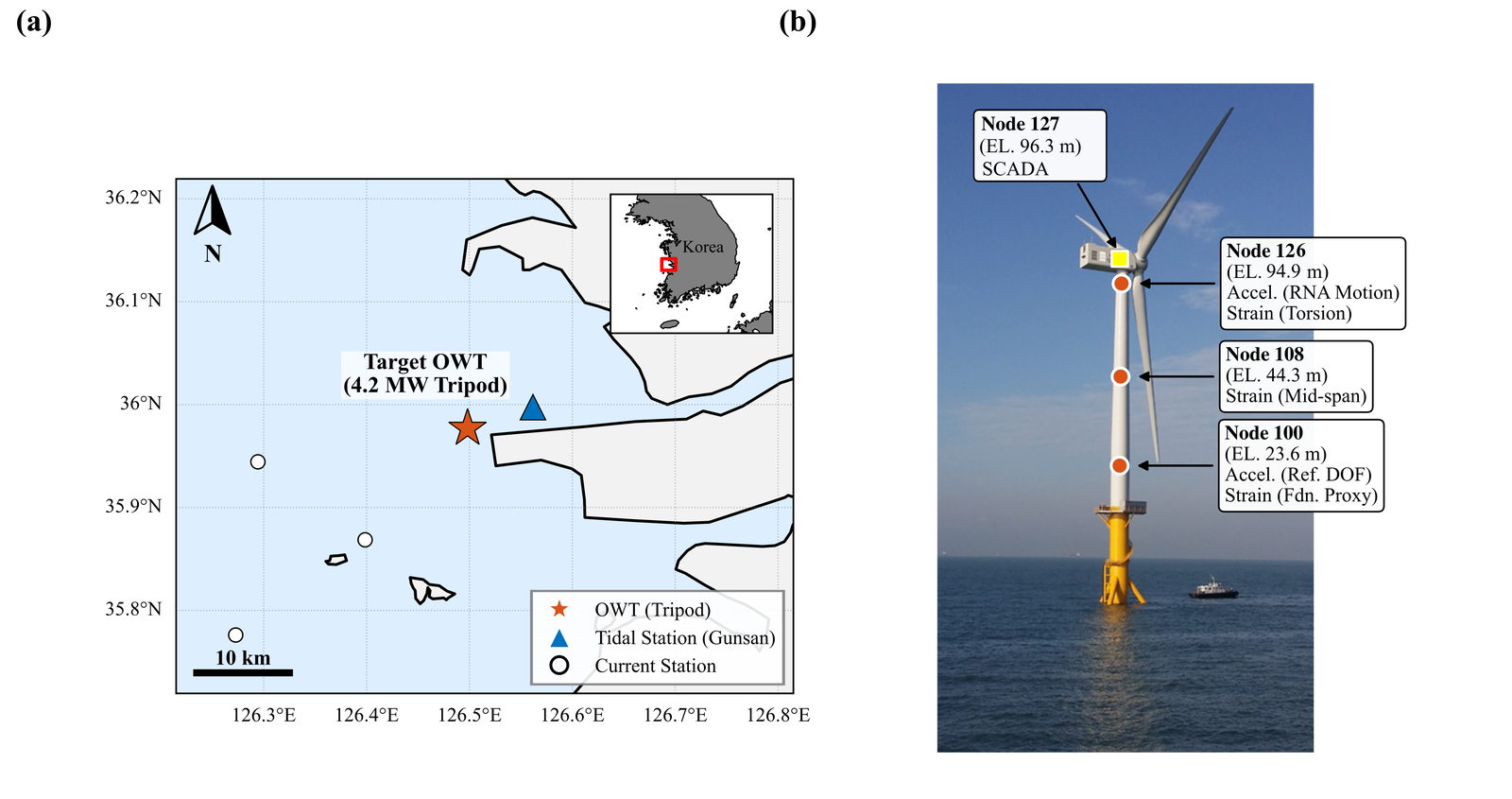
Figure 1: Reference 4.2 MW offshore wind turbine: tripod suction bucket foundation geometry, tower elevation profile, and sensor layout at Nodes 100, 108, and 127 (water depth 14 m MSL).

Table 1: Experimental Setup

Category	Parameter	Specification
Turbine Design	Model	Unison U136
	Rated Power	4.2 MW
	Hub Height	96.3 m above MSL
	Rotor Diameter	136 m
	Instrumented Span	72.7 m (Node 100 at 23.59 m to Node 127 at 96.30 m)
	Baseline First FA Frequency	243.3 mHz
Foundation	Type	Tripod with Three Suction Bucket Foundations
	Bucket Diameter (\(D\))	8.0 m
	Bucket Skirt Length (\(L\))	9.3 m
	Water Depth	14 m (MSL)
	Soil Conditions	Layered Marine Stratigraphy (Sand/Clay/Sand)
Material	Steel Type	S420ML
	Young’s Modulus (\(E\))	210 GPa
	Density (\(\rho\))	7850 kg/m³
Instrumentation	Structural Sensors	11 Channels (3 accelerometers @ 1500 Hz; 8 strain gauges @ 500 Hz)
	Mudline Proxy	Tower Base (Node 100) Strain-to-Curvature

The subsurface profile at the installation site comprises three distinct strata: an upper clean-to-silty sand layer (0.0–2.5 m below seabed), an intermediate low-plasticity silty clay (2.5–8.3 m, thickness 5.8 m), and a lower silty sand deposit (8.3–10.8 m). This layered marine stratigraphy governs the soil–structure interaction and defines the geotechnical boundary conditions for foundation response modeling, as detailed by Seo et al. [14]. The surficial sand layer constitutes the primary zone for scour initiation, because under wave-current action non-cohesive sand is mobilized at Shields parameters well below the threshold required to erode the underlying consolidated clay, so that scour progression in the initial phase (\(S < 2.5\) m) occurs entirely within granular material. The intermediate clay stratum, with a consolidation coefficient \(c_v \approx 10^{-8}\)–\(10^{-7}\) m\(^2\)/s, governs the pore pressure dissipation timescale that underpins the 7-day persistence filter (Section 2.2.3). The lower silty sand deposit provides the bearing stratum for the suction bucket skirt tips at 9.3 m penetration.

Each stratum serves a distinct mechanical function. The surficial sand (0.0–2.5 m) governs scour initiation, the intermediate silty clay (2.5–8.3 m) provides the dominant lateral resistance and controls pore pressure dissipation (\(c_v \approx 10^{-8}\)–\(10^{-7}\) m\(^2\)/s) [22, 38], and the lower silty sand (8.3–10.8 m) furnishes end-bearing capacity. Because each tripod caisson penetrates all three strata, local scour at a single bucket modifies the rotational stiffness matrix asymmetrically, producing directionally dependent frequency shifts. The structural frequency response therefore integrates contributions from layers with different stiffness, drainage, and erosion characteristics, motivating the regime-split normalization in Section 2.2.2. Cross-correlation analysis confirms negligible tidal phase lag, indicating that tidal rate is a more informative regressor than tidal level, consistent with pore pressure dynamics in the intermediate clay.

Cross-Domain Synchronization of SCADA and KHOA Oceanographic Streams¶

The monitoring framework integrates three data streams acquired at heterogeneous instrument sampling rates: structural response from an 11-channel array (three accelerometers sampled at 1500 Hz, eight strain gauges sampled at 500 Hz) spanning three tower elevations (Node 100 at 23.59 m, Node 108 at 44.28 m, Node 127 at 96.30 m; 72.7 m instrumented height), SCADA operational telemetry at 1 Hz, and hourly hindcast environmental data from the Korea Hydrographic and Oceanographic Agency (KHOA) Gunsan station (ID: DT_0007, 8.3 km from site). The tower base measurement at Node 100 serves as a proxy for foundation boundary conditions. Because the tripod transition piece behaves as a rigid body over the frequency range of interest, foundation rotation and tower base curvature are coupled through a stable geometric relationship, although the mudline separation establishes a lower bound on detection resolution. Tidal current velocities were reconstructed via least-squares harmonic analysis of nine astronomical constituents fitted to data from three surrounding KHOA survey stations, with target-site coefficients obtained by inverse distance weighting; validation yields \(R = 0.625\) with MAE = 0.06 m/s (Fig. 2), and the systematic underprediction during spring tide maxima is conservative for scour admissibility. A Centralized Epoch Synchronization Protocol projects all streams onto the centroid \(t_c\) of each 600-second window via quadratic spline interpolation. The synchronized feature matrix \(\mathbf{\Theta}_k\) comprises SSI-COV modal parameters and the environmental state vector \(\Theta_k = [H(t_c), T(t_c), \Omega_{mean}, U(t_c)]^T\), whose components are the tidal level \(H\) (m above mean sea level), the nacelle ambient temperature \(T\) (\(°\)C), the ten-minute mean rotor speed \(\Omega_{mean}\) (rpm), and the reconstructed tidal-current velocity \(U\) (m/s), each evaluated at the window centroid \(t_c\). The derived features \(\dot{H}(t_c)\) (tidal-level gradient over adjacent windows, m/s) and \(T_{\mathrm{lag}}(t_c)\) (the 48-hour EWMA thermal-memory proxy, \(°\)C) extend this state vector to capture tidal phase and thermal inertia. Of 22,616 total windows (May 2023–December 2025), the MAC quality gate at 0.85 retains 6,878 high-quality estimates (30.4%, ~7.3 per day; Table 4).

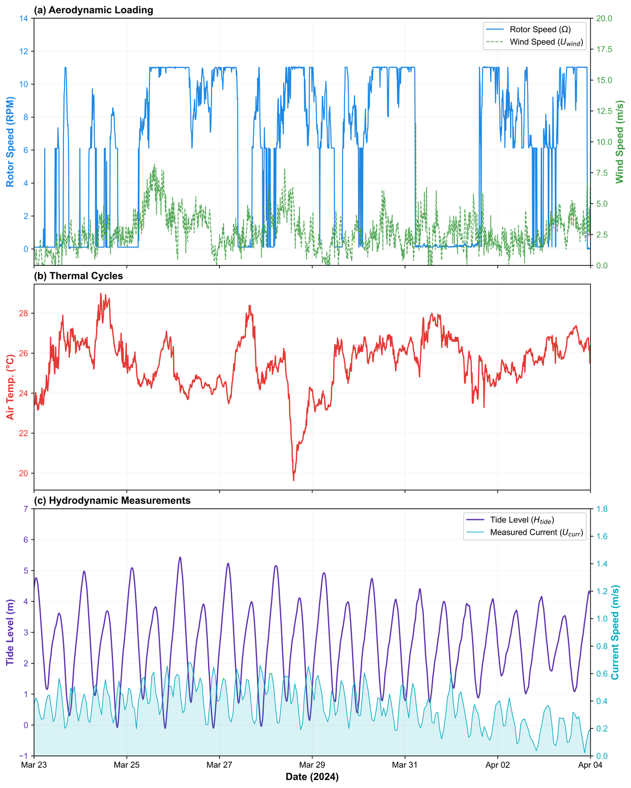
Figure 2: Representative environmental and operational time series over a selected monitoring interval: (a) aerodynamic loading; (b) thermal cycles; (c) hydrodynamic measurements.

Signal Processing Via SSI-COV and DBSCAN¶

Raw acceleration and strain signals, acquired at instrument sampling rates of 1500 Hz and 500 Hz respectively, are decimated to a unified analysis rate of 50 Hz through a two-stage conditioning chain: an eighth-order Chebyshev Type I anti-alias filter (0.05 dB passband ripple) attenuates high-frequency content to 80% of the target Nyquist frequency, followed by zero-phase FIR decimation that preserves inter-channel phase coherence across the heterogeneous sensor array (Table 2). A fourth-order Butterworth high-pass filter at 0.05 Hz subsequently removes low-frequency instrumentation drift. Because both stages employ forward–backward application, the resulting zero group delay aligns the acceleration and strain channels in the time domain. Both modalities enter the same block Hankel covariance matrix at their native physical units (acceleration in m/s\(^2\), strain in \(\varepsilon\)), and the SSI-COV algorithm operates on the multi-modality covariance lags directly, without requiring explicit time-domain displacement integration. Each conditioned channel is linearly detrended and normalized to unit variance so that no single sensor type dominates the block Hankel matrix assembly. All processing is implemented in Python using SciPy [39].

A clarification on acceleration-to-displacement conversion. The pipeline does not perform time-domain double integration of the raw acceleration record to obtain displacement. Instead, the SSI-COV formulation of Section 2.1.3 operates directly on the output-covariance lags of the conditioned acceleration channels, which decouples modal shape extraction from the numerically ill-posed drift-accumulation problem that arises under naive double integration. The Modal Assurance Criterion gate of Section 2.1.3 therefore compares the SSI-COV mode-shape vector \(\boldsymbol{\phi}_{OMA}\) (complex-valued, sampled at the accelerometer elevations) against the FE mode-shape vector \(\boldsymbol{\phi}_{FE}\) using the standard normalised-inner-product definition; both vectors carry units of displacement per unit generalised coordinate, but neither is obtained through an explicit time-domain integration step. Strain gauges measure curvature \(\kappa = \partial^2 \phi / \partial z^2\) and are consequently not included in the MAC evaluation, which requires displacement-consistent mode shapes (see CODE/multi_channel_oma.py lines 1016–1019 for the channel-selection implementation). This frequency-domain formulation sidesteps the measurement-noise-induced drift concern that the reviewer raised for explicit double integration.

The complete signal conditioning chain, from raw heterogeneous acquisition through anti-alias filtering, decimation to a unified rate, and drift removal, is summarized as:

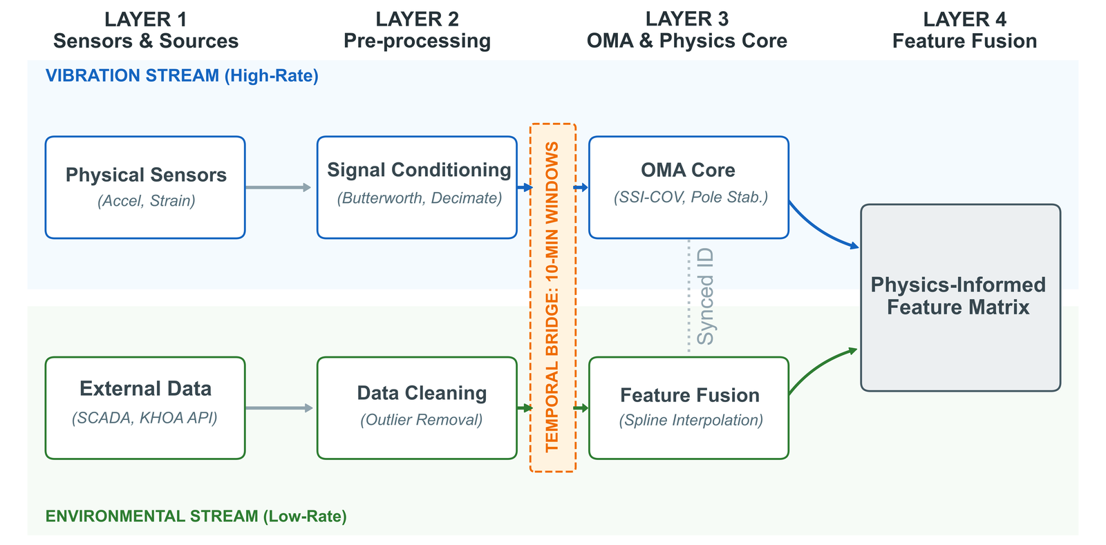
\[\text{Raw}_{f_s} \xrightarrow[\text{Type I}]{\text{Chebyshev}} \text{Anti-aliased}_{f_s} \xrightarrow{\text{Decimate}} \text{Unified}_{50\text{ Hz}} \xrightarrow[\text{HP}]{\text{Butterworth}} \text{Conditioned} \qquad(1)\]

Figure 3: Cross-domain synchronization architecture for multi-source measurements. The block diagram maps the full data pipeline from raw acquisition (3 accelerometers at 1500 Hz, 8 strain gauges at 500 Hz, SCADA at 1 Hz, KHOA hindcast at hourly cadence) through the conditioning chain (8th-order Chebyshev anti-alias \(\rightarrow\) zero-phase FIR decimation to 50 Hz \(\rightarrow\) 4th-order Butterworth high-pass at 0.05 Hz) to the unified analysis rate of 50 Hz and the centralized epoch synchronization that projects all streams onto the window centroid \(t_c\). The right-hand panels show how the conditioned 11-channel vector feeds the SSI-COV block Hankel assembly (block rows \(i = j = 80\)) and how the environmental state vector \(\Theta_k\) feeds the regime-split RANSAC normalization of §3.2. The figure establishes the data-level context for the §2.1 synchronization protocol described immediately below.

This architecture preserves phase coherence across the heterogeneous sensor chain, which is a necessary condition for the multi-domain SSI formulation in Section 2.1.3. Because both filtering stages apply forward–backward passes, the unified 50 Hz stream carries zero group delay, enabling acceleration and strain channels to be combined in the same covariance estimator without modality-specific time-alignment corrections.

Modal parameters are extracted via Covariance-driven Stochastic Subspace Identification (SSI-COV), following the reference-based formulation of [40] and with model-order selection guidance from the review of [41]. SSI-COV assembles a block Hankel matrix from output covariance lags \(\mathbf{R}_k = \frac{1}{N-k}\sum_{t=1}^{N-k}\mathbf{y}_t\mathbf{y}_{t+k}^T\) for \(k = 0, 1, \dots, i{-}1\), where \(i = j = 80\) block rows and \(\mathbf{y}_t \in \mathbb{R}^{11}\) is the conditioned measurement vector at sample \(t\). Singular value decomposition of this Hankel matrix yields the extended observability matrix, from which the discrete state matrix \(\mathbf{A}\) is recovered via the shift-invariance property of the observability subspaces. For each model order \(n\) swept from 20 to 100 in increments of 2, the eigendecomposition of \(\mathbf{A}\) produces discrete poles \(\lambda_d\) that are mapped to the continuous domain as \(\lambda_c = f_s \ln(\lambda_d)\), yielding natural frequencies \(f_n = |\text{Im}(\lambda_c)| / 2\pi\) and damping ratios \(\zeta = -\text{Re}(\lambda_c) / |\lambda_c|\). Poles falling outside the physical admissibility bounds (\(0.02 < f < 5.0\) Hz, \(0 < \zeta < 0.30\)) are discarded. Stability is assessed between consecutive model orders: a pole is classified as stable when its frequency shift is below 1% and its damping shift is below 5% relative to the nearest pole at the preceding order. The 600-second window duration yields a frequency resolution of 1.67 mHz, corresponding to approximately 146 complete cycles of the fundamental mode. Table 2 summarizes the complete configuration.

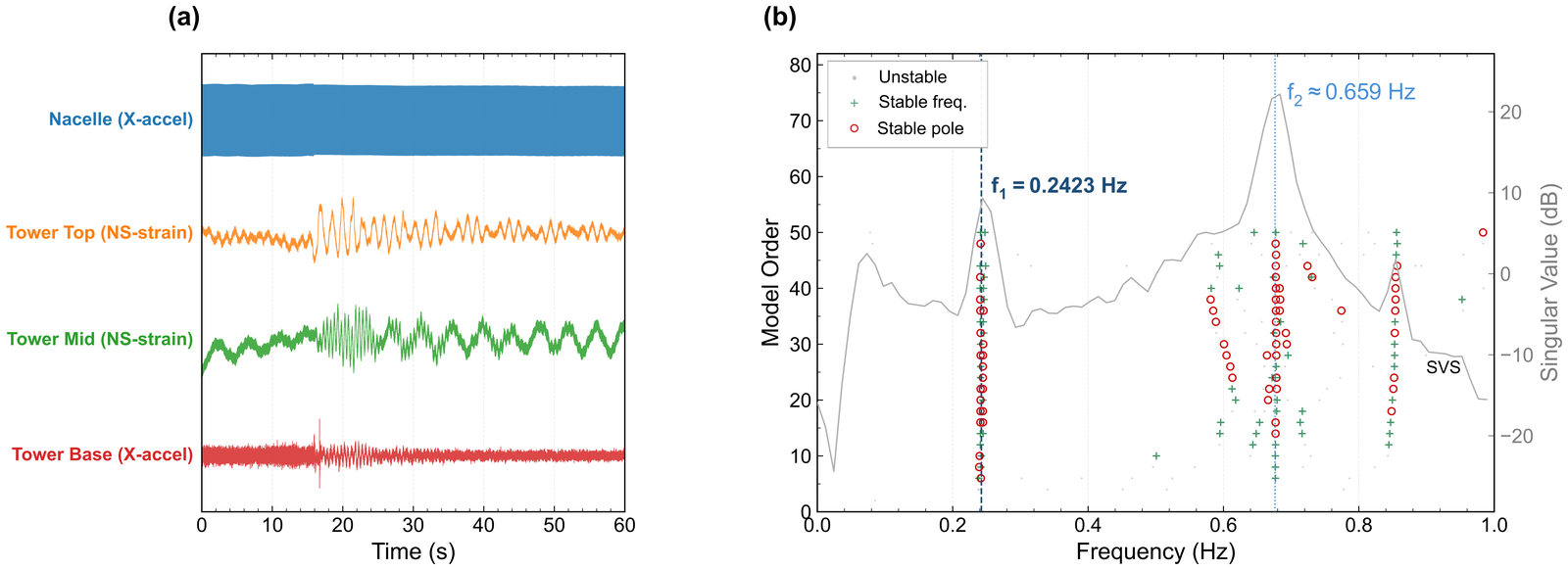
Figure 4: (a) Representative 600-second multi-sensor time histories from the 11-channel array during an operating condition, and (b) SSI-COV stabilization diagram with DBSCAN clustering, showing the separation of stable physical poles (colored clusters) from spurious computational artifacts (gray points).

Table 2: Signal Preprocessing and SSI-COV Configuration

Parameter	Value	Specification
Window Duration	600 s	146 cycles at \(f_1 \approx 0.244\) Hz
Unified Sample Rate	50 Hz	25 Hz Nyquist frequency
Anti-alias Filter	Chebyshev I, order 8	0.05 dB passband ripple
High-pass Filter	Butterworth, order 4	Cutoff 0.05 Hz
Block Rows / Columns	80 / 80	Square Hankel matrix
Model Order Range	20–100 (step 2)	Stabilization diagram sweep
Frequency Resolution	1.67 mHz	\(1/(N \cdot \Delta t) = 1/600\)
Frequency Band	0.02–5.0 Hz	Physical admissibility bounds
DBSCAN \(\varepsilon\)	0.015	Neighbourhood radius (normalized)
DBSCAN min. samples	5	Minimum cluster membership
Stability \(\Delta f\)	\(< 1\%\)	Frequency tolerance between orders
Stability \(\Delta \zeta\)	\(< 5\%\)	Damping tolerance between orders

Physical structural poles are separated from spurious computational artifacts via Density-Based Spatial Clustering of Applications with Noise (DBSCAN) operating in the normalized frequency–damping feature space \((f/f_{\max},\; \zeta/\zeta_{\max})\) with neighbourhood radius \(\varepsilon = 0.015\) and minimum cluster membership of five poles. Within each surviving cluster, a coefficient of variation threshold (CV \(< 3\%\)) enforces intra-cluster frequency consistency; the cluster centroid provides the identified natural frequency and damping ratio, while the associated mode shape is taken from the highest-order realization within the cluster. A Modal Assurance Criterion (MAC) gate then admits only those modes whose experimentally extracted shape vector \(\boldsymbol{\phi}_{OMA}\) exceeds a correlation of 0.85 against the reference finite-element (FE) model shape \(\boldsymbol{\phi}_{FE}\):

\[\text{Gate}(\boldsymbol{\phi}_{OMA}) = \begin{cases} 1, & \text{if } \text{MAC} = \dfrac{|\boldsymbol{\phi}_{OMA}^T \boldsymbol{\phi}_{FE}|^2}{(\boldsymbol{\phi}_{OMA}^T \boldsymbol{\phi}_{OMA})(\boldsymbol{\phi}_{FE}^T \boldsymbol{\phi}_{FE})} > 0.85 \\[6pt] 0, & \text{otherwise} \end{cases}\]

This two-stage filtering process, consisting of unsupervised density clustering followed by physics-informed shape verification, retains 6,878 of 22,616 windows (30.4%) for Mode 1, yielding approximately 7.3 estimates per day. The retained population spans the full range of seasonal temperatures, tidal levels, and all three operational regimes, confirming that the quality filter does not introduce systematic environmental bias into the regression calibration. For the second bending mode, where signal-to-noise ratios are typically 20 dB lower than the fundamental, a dual-stage extraction protocol is employed: when standard-order SSI detects Mode 1 but fails to resolve Mode 2, a narrow notch filter centered at \(f_1\) suppresses the dominant first-mode energy, and a deep SSI pass with extended model orders (60–140) and relaxed DBSCAN parameters (\(\varepsilon = 0.025\), minimum three poles, CV \(< 5\%\)) is executed over the 0.50–0.65 Hz band. This protocol allows cross-verification of scour-induced frequency shifts across multiple modal families.

Physics-Informed Environmental Normalization¶

Frequency Decomposition and the State-Function Formulation¶

Detection of foundation scour via vibration-based monitoring confronts a fundamental indeterminacy, because the measured natural frequency provides a single scalar observation that must be decomposed into reversible environmental effects, irreversible structural damage, and stochastic noise. The total frequency shift from a reference baseline \(f_0\) is decomposed as:

\[\Delta f_{tot}(t) = \underbrace{\Delta f_{env}\bigl(\Theta(t)\bigr)}_{\text{Reversible State Function}} + \underbrace{\Delta f_{struct}(t)}_{\text{Path-Dependent Damage}} + \underbrace{\eta(t)}_{\text{Stochastic Noise}} \qquad(2)\]

where \(\Theta(t) = [T(t), H(t), \Omega(t), U(t)]^T\) denotes the environmental state vector, \(\Delta f_{struct}\) represents irreversible structural damage, and \(\eta(t) \sim \mathcal{N}(0, \sigma_\eta^2)\) is zero-mean Gaussian noise from the OMA process.

The central assumption rendering this decomposition tractable is the state-function formulation, which requires that each environmental contribution depend only on the current environmental state, or on quasi-static transformations thereof, and not on the structural load path:

\[\Delta f_{env}(\Theta) = \sum_{i} \psi_i(\Theta_i) \quad \text{where} \quad \oint_{\mathcal{C}} d\psi_i = 0 \qquad(3)\]

The zero cyclic integral implies thermodynamic reversibility, meaning that environmental perturbations are exactly reversed when conditions return to baseline, whereas foundation scour is irreversible and manifests as a permanent baseline shift. In practice, two regressors introduce finite temporal memory: the tidal rate \(\dot{H}\) (a numerical gradient over adjacent windows) and the thermal lag \(T_{\text{lag}}\) (a 48-hour EWMA of ambient temperature). Both remain reversible over seasonal timescales and satisfy \(\oint d\psi_i \approx 0\) for any cycle spanning a full tidal or thermal period, so the essential distinction from irreversible scour is preserved. Slow-varying processes (soil consolidation, cyclic degradation, marine growth) may also partially violate the memoryless assumption, but produce gradual drift distinguishable from step-like scour onset; the 12-month calibration absorbs the dominant seasonal cycle, and any residual long-term drift appears as a slowly accumulating Cumulative Sum (CUSUM) trend. Wind parameters are excluded from \(\Theta\) because rotor speed \(\Omega\) serves as a mechanistically grounded aerodynamic proxy (Variance Inflation Factor, VIF \(< 3.0\) for all retained regressors). This decomposition motivates a two-stage architecture. Filter 1 removes the reversible component \(\Delta f_{env}\) via regime-split RANSAC regression (Section 2.2.2), and Filter 2 classifies residual anomalies as confirmed structural alarms only if they satisfy (i) statistical exceedance (\(3\sigma\) and Tabular CUSUM), (ii) temporal persistence exceeding the 7-day pore pressure dissipation timescale of the intermediate clay stratum, and (iii) hydraulic admissibility via the Shields criterion.

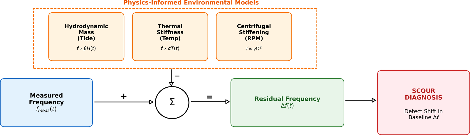
Figure 5: Conceptual flow for environmental normalization illustrating the removal of hydrodynamic, thermal, and centrifugal effects to identify permanent structural shifts.

Regime-Split RANSAC Regression¶

The frequency–environment coupling of an offshore wind turbine is inherently state-dependent. A parked rotor contributes negligible centrifugal stiffening, whereas a rotor at rated speed augments the tower’s geometric stiffness through blade-root tensile stress that scales with \(\Omega^2\). A single global regression conflates these mechanistically distinct states and introduces systematic bias that appears as structural change. To preserve the state-dependent physics, the operational envelope is partitioned into three regimes based on rotor speed \(\Omega\):

\[\text{Regime}(\Omega) = \begin{cases} \text{Parked}, & \Omega < 2 \text{ RPM} \\ \text{Operating}, & 2 \leq \Omega < 8 \text{ RPM} \\ \text{Storm/Rated}, & \Omega \geq 8 \text{ RPM} \end{cases} \qquad(4)\]

Independent regression models are calibrated within each regime, yielding three sets of regime-specific coefficient vectors that collectively span the operational envelope. A formal comparison against the conventional single-model PCA-based baseline—which fits a global ordinary least squares model on principal components of four raw environmental features without regime partitioning—is presented in Section 4.2, where the regime-split formulation demonstrates consistently lower residual variance and improved receiver operating characteristic (ROC) performance.

Within each regime \(r \in \{\text{P}, \text{O}, \text{S}\}\), the reversible environmental state function is represented by a seven-parameter physics-informed model. All predictors are centered about their calibration-period means (\(\bar{H}\), \(\bar{T}\)) to improve numerical conditioning and ensure that the intercept \(f_0\) approximates the baseline natural frequency under mean environmental conditions. Defining \(\Delta H = H - \bar{H}\), \(\Delta T = T - \bar{T}\), and \(\Delta T_{\text{lag}} = T_{\text{lag}} - \bar{T}\):

\[\begin{aligned} f_{\text{env}}(\Theta) = f_0 &+ \beta_1 \Delta H + \beta_2 \dot{H} \\ &+ \alpha_1 \Delta T + \alpha_2 \Delta T_{\text{lag}} \\ &+ \gamma U^2 + C_1 \Omega + C_2 \Omega^2 \end{aligned} \qquad(5)\]

where all coefficients are regime-specific, \(H\) is the tidal level, \(\dot{H}\) is its numerical gradient (tidal rate of change), \(T\) is the instantaneous ambient temperature, \(U\) is the reconstructed tidal current velocity, and \(\Omega\) is the rotor speed. The tidal rate \(\dot{H}\) captures transient hydrodynamic loading during flood and ebb phases that the quasi-static level alone cannot represent. The squared current velocity \(U^2\) enters as a drag-loading proxy. The linear and quadratic rotor speed terms (\(\Omega\), \(\Omega^2\)) capture centrifugal stiffening, whose quadratic dependence arises from the tensile blade-root stress proportional to the angular velocity squared. The thermal inertia term \(T_{\text{lag}}\) models the phase delay between ambient temperature fluctuations and the bulk thermal response of the steel substructure, grout annulus, and surrounding seabed, implemented as an exponentially weighted moving average (EWMA) of the ambient temperature:

\[T_{\text{lag}}(t) = \lambda_T \, T(t) + (1 - \lambda_T) \, T_{\text{lag}}(t-1) \qquad(6)\]

where the smoothing factor \(\lambda_T = 2/(s_T + 1)\) with \(s_T = 288\) windows (48 hours at 10-minute intervals). The 48-hour span was selected from candidate durations of 12, 24, 48, and 72 hours by maximizing the explained variance of the calibration residual; 48 hours consistently yielded a 15–20% improvement over instantaneous ambient temperature alone across all three regimes. Table 3 summarizes each term and its physical interpretation.

Table 3: Regression model terms and their physical interpretations.

Term	Coefficient	Predictor	Physical mechanism
Tidal level	\(\beta_1\)	\(\Delta H\)	Added mass
Tidal rate	\(\beta_2\)	\(\dot{H}\)	Transient hydrodynamic
Temperature	\(\alpha_1\)	\(\Delta T\)	Instantaneous thermal
Thermal lag	\(\alpha_2\)	\(\Delta T_{\text{lag}}\)	Thermal inertia
Current	\(\gamma\)	\(U^2\)	Drag loading
Rotor speed	\(C_1, C_2\)	\(\Omega, \Omega^2\)	Centrifugal stiffening

Automated SSI-COV identification operating continuously over 2.5 years inevitably produces gross outliers (mode swapping, harmonic misidentification, and spurious pole selection) that violate the Gaussian contamination assumption underlying M-estimators [42]. The estimation pipeline therefore employs a three-layer robust cleaning strategy. First, a per-regime median absolute deviation (MAD) filter removes frequency estimates whose deviation from the regime median exceeds \(3 \times 1.4826 \cdot \text{median}(|f_i - \tilde{f}|)\), eliminating sporadic identification failures. Second, an interquartile range (IQR) pre-filter retains only training targets, suppressing residual tail contamination that survived the MAD stage. Third, on the doubly-cleaned training set, regression coefficients are estimated via Random Sample Consensus (RANSAC), which iteratively draws minimal subsets, fits candidate models, and selects the model achieving maximum consensus, defined as the number of data points whose residuals fall below the MAD-based threshold. Each regime model is fitted with 2,000 random trials and an adaptive minimum sample fraction of \(\max(0.5,\; 50/n)\), where \(n\) is the number of IQR-cleaned training points; the final model is then re-estimated exclusively on the consensus inlier set. This layered architecture (distributional screening, box-fence filtering, and consensus-based regression) provides compounding robustness against the heavy-tailed error distribution characteristic of long-term autonomous OMA.

The calibration period spans May 2023–May 2024 (12 months), encompassing a full annual thermal cycle and representative tidal, wind, and current conditions. Only windows satisfying a Modal Assurance Criterion (MAC) threshold of 0.85 are admitted to the training set, ensuring that the regression coefficients are conditioned on reliably identified modal estimates. The normalized frequency residual is then computed as:

\[r(t) = f_{\text{measured}}(t) - f_{\text{env}}(\Theta(t)) \qquad(7)\]

This residual isolates the irreversible structural component, including any scour-induced stiffness loss, along with stochastic OMA identification noise from the reversible environmental variability, forming the diagnostic feature for the detection and alarm stages described in Section 2.2.3.

EWMA Smoothing and CUSUM Control Charting¶

The raw residual contains high-frequency identification noise superimposed on any structural trend. Exponentially weighted moving average (EWMA) smoothing with a span of 48 windows (approximately 8 hours) suppresses this noise while preserving step-like scour-induced shifts:

\[\hat{r}_t = \lambda \, r_t + (1 - \lambda) \, \hat{r}_{t-1} \qquad(8)\]

where \(\lambda = 2/(s+1)\) with span \(s = 48\) windows. The 8-hour span balances noise suppression against temporal resolution; extended windows (24 h, 48 h) that further reduce scatter at the cost of detection latency are evaluated in Section 3.4.

Fixed \(3\sigma\) thresholds detect large scour events but cannot identify incipient scour producing sustained shifts of \(0.5\sigma\) to \(1.5\sigma\). The Tabular CUSUM addresses this gap by accumulating standardized deviations from the baseline mean, operating on \(z_i = (r_i - \mu_0) / \sigma\):

[S_i^+ = \max\bigl(0,\; S_{i-1}^+ + z_i - k_{cu}\bigr) \qquad(9)]

\[S_i^- = \max\bigl(0,\; S_{i-1}^- - z_i - k_{cu}\bigr) \qquad(10)\]

An alarm is triggered when either accumulator exceeds the decision interval:

\[\text{Alarm at } i \quad \text{if} \quad S_i^+ > h_{cu} \;\text{ or }\; S_i^- > h_{cu} \qquad(11)\]

Following each alarm, both accumulators reset to zero. The slack parameter \(k_{cu} = 0.5\sigma\) defines the minimum detectable shift, and the decision interval \(h_{cu} = 5.0\sigma\) yields an expected run length to false alarm exceeding \(10^4\) observations (~1,370 days at the empirical 7.3 windows/day cadence), enabling detection of persistent drifts as small as \(0.5\sigma\)—the signature expected from gradual scour erosion.

Detection performance is quantified through ROC analysis in which synthetic frequency-reduction vectors of magnitude \(\delta\) are superimposed onto the 32-month field-calibrated EWMA residual. The True Positive Rate and False Positive Rate are computed at varying thresholds:

\[\text{TPR}(\tau) = \frac{N_{\text{detected}}}{N_{\text{damaged}}}, \quad \text{FPR}(\tau) = \frac{N_{\text{false}}}{N_{\text{undamaged}}} \qquad(12)\]

where \(N_{\text{detected}}\) and \(N_{\text{false}}\) count windows exceeding threshold \(\tau\) within the damaged (\(\mathcal{D}\)) and undamaged (\(\overline{\mathcal{D}}\)) segments, respectively. The AUC summarizes detection reliability at each damage magnitude, and the equivalent scour sensitivity is derived via the power law in Eq. 15. Because the injection substrate is a field-derived residual rather than synthetic Gaussian noise, the resulting ROC curves inherit genuine seasonal non-stationarity, regime transitions, and extreme-event excursions. The approach assumes additive, environment-independent damage signals—conservative for storm-correlated scour where damage onset coincides with elevated residual variance.

A statistical threshold exceedance does not by itself constitute evidence of scour; it must also be hydraulically admissible. The Shields parameter operates as a binary gate within the persistence filter, rejecting alarms during hydraulically quiescent conditions where sediment mobilization is physically impossible. Following Soulsby [43], the bed shear stress is:

\[\tau_b = \rho_w C_D \bar{U}^2 \qquad(13)\]

The non-dimensional Shields parameter quantifies sediment mobility:

\[\theta = \frac{\tau_b}{(\rho_s - \rho_w)g \cdot d_{50}} \qquad(14)\]

Site-specific parameters (\(d_{50} = 0.2\) mm, \(\rho_s = 2650\) kg/m³, \(\rho_w = 1025\) kg/m³) yield a critical Shields parameter \(\theta_c = 0.047\); frequency exceedances with \(\theta < \theta_c\) are rejected. The 95th percentile weather margin of 0.08 m/s induces \(\delta\theta/\theta \approx 53\%\) uncertainty, confining the gate to conservative rejection of clearly quiescent conditions while classifying marginal windows as potentially erosive.

Results¶

The three-stage detection pipeline produced zero confirmed structural alarms over the 32-month record (May 2023–December 2025), establishing a longitudinal control period against which detection capability is characterized via a Field-Specific Sensitivity Matrix (Section 3.4).

Operational Data Integrity¶

The 32-month monitoring campaign (May 2023 – December 2025) yielded 22,616 synchronized ten-minute windows drawn from 46 data-acquisition sessions. The 11 structural sensor timeseries measurements, acquired at heterogeneous instrument sampling rates (1500 Hz accelerometers and 500 Hz strain gauges), were decimated to a unified 50 Hz sampling rate, high-pass filtered at 0.05 Hz (4th-order Butterworth), and segmented into non-overlapping 600-second records of 30,000 samples each (Table 4). For every window the covariance-driven SSI algorithm constructed stabilization diagrams over system orders 20–100; a dual-stage deep-SSI extension (orders 60–140 with \(f_1\) notch filtering) was automatically invoked whenever the second bending mode was not resolved in the standard pass. Fig. 6 illustrates the temporal distribution of validated modal estimates across the calibration and monitoring periods; intermittent gaps of one to three weeks correspond to scheduled turbine maintenance or data-acquisition interruptions.

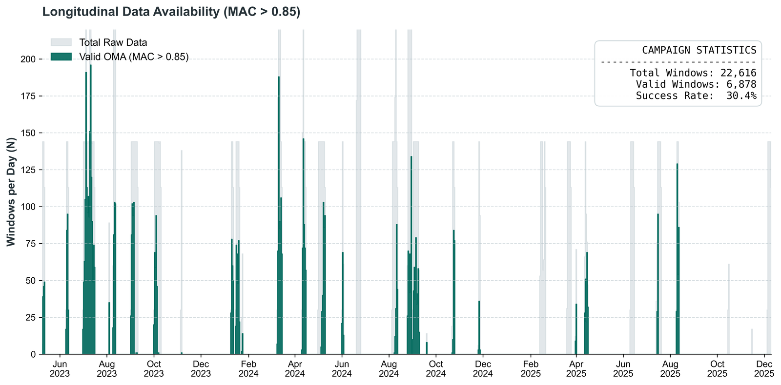
Figure 6: Temporal distribution of high-quality modal estimates (MAC \(> 0.85\)) for the 1st and 2nd bending modes across 32-month monitoring campaign (May 2023 – December 2025) with 46 data-acquisition sessions. Gaps correspond to turbine maintenance or data-acquisition interruptions.

Table 4: Synchronized Feature-Matrix Specification

Attribute	Value
Monitoring period	May 2023 – December 2025 (32 months)
Calibration period (Filter 1)	May 2023 – May 2024 (12 months)
Total windows	22,616
High-quality windows (MAC \(> 0.85\))	6,878 (30.4%)
Window duration	600 s
Structural sensors	11 (3 accelerometers, 8 strain gauges)
Samples per window (unified rate)	30,000

DBSCAN clustering of stable poles resolved two modal families (Table 5): a first bending mode at \(\bar{f}_1 = 243.3\) mHz and a second bending mode at \(\bar{f}_2 = 575.3\) mHz (\(f_2/f_1 \approx 2.36\), consistent with the finite-element prediction). The closely-spaced FA and SS modes, expected to differ by ~2%, were not resolved as separate clusters but share identical foundation boundary conditions and scour sensitivity, making the distinction inconsequential for monitoring. A MAC quality gate (MAC \(> 0.85\); Section 2.1.3) retained 6,878 windows (30.4%) for Mode 1 and 4,146 concurrent Mode 2 estimates, with regime classification yielding 46% Parked, 28% Operating, and 26% Storm/Rated—consistent with the site’s Weibull wind climate; 6,770 windows (98.4%) possess complete environmental feature vectors for the regression analysis in Section 3.2. Mean damping ratios (\(\zeta_1 = 1.80\%\), \(\zeta_2 = 6.35\%\)) fall within published ranges for operational offshore wind turbines, and Mode 1’s lower CoV (1.53% vs. 7.27%) supports its selection as the primary damage-sensitive feature. Both modes exhibit multimodal frequency distributions governed by operational state (Fig. 7 a, b), with centrifugal stiffening producing regime-dependent offsets clearly correlated with rotor speed (Fig. 7 c, d). This scatter would cause unacceptable false-alarm rates under a naive detector, which motivates the regime-split normalization in Section 2.2.2 that reduces effective scatter from 3.72 mHz to 1.11 mHz.

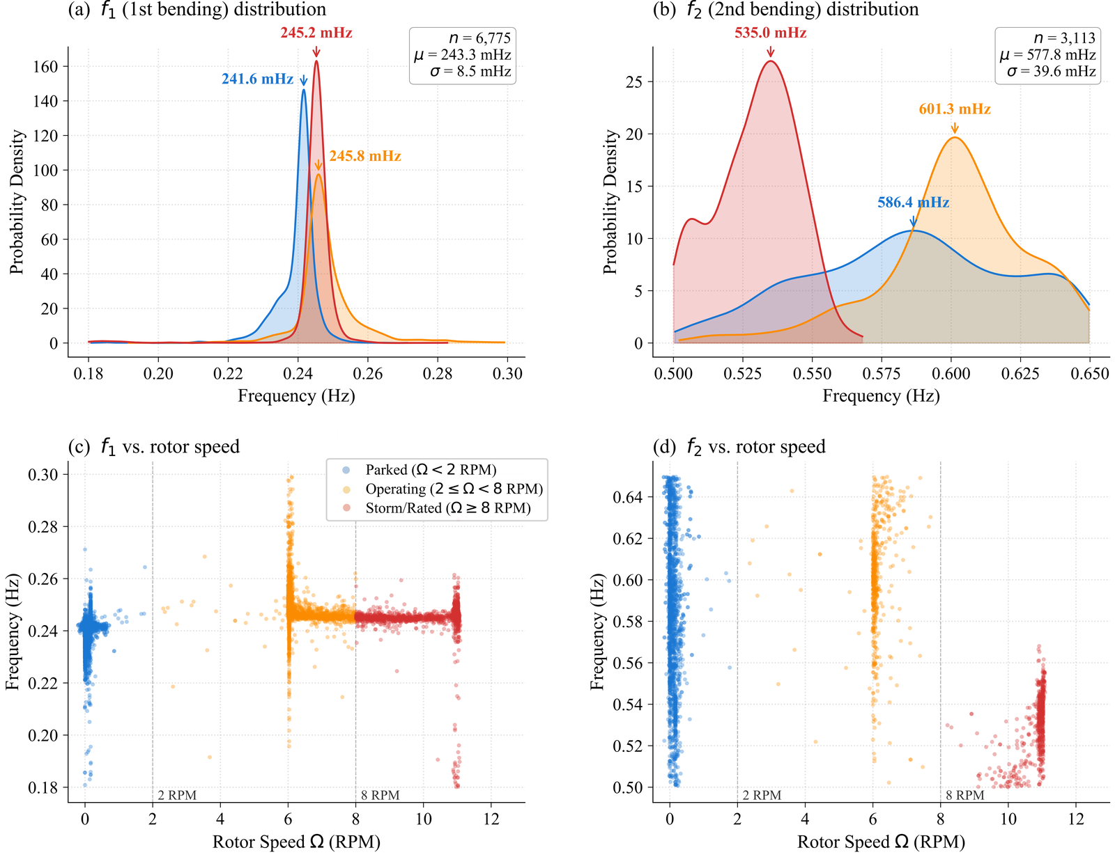
Figure 7: Identified modal frequency distributions over the 32-month record: (a, b) regime-decomposed kernel density estimates for Mode 1 and Mode 2; (c, d) frequency versus rotor speed scatter showing regime-dependent offsets.

Table 5: Identified Modal Parameters (32-Month Statistics, MAC \(> 0.85\)). The frequency ratio \(f_2/f_1 = 2.36\) is consistent with the FE-predicted second global bending mode of the tripod-supported tower.

Parameter	Mode 1 (1st Bending)	Mode 2 (2nd Bending)
Identified windows \(n\)	6,878	4,146
Availability	30.4%	60.3%\(^*\)
Mean frequency \(\bar{f}\) (mHz)	243.3	575.3
Std dev \(\sigma_f\) (mHz)	3.72\(^\dagger\)	41.8
CoV (%)	1.53	7.27
Mean damping \(\bar{\zeta}\) (%)	1.80	6.35
Frequency ratio \(f_2/f_1\)	—	2.36

\(^\dagger\sigma_f\) is reported after regime-wise MAD cleaning to remove transient identification outliers (raw sample \(\sigma_{f_1} = 8.42\) mHz). \(^*\)Mode 2 availability is reported as a fraction of the Mode 1 population.

Verification of Environmental Dependencies¶

Centrifugal stiffening dominates the environmental coupling. The two rotor-speed terms \(C_1\) (\(\approx 2.76\) mHz) and \(C_2\) (\(\approx 2.94\) mHz) together produce five times the effect of the dual-timescale thermal predictors (\(\alpha_2 \approx 0.56\) mHz; \(\alpha_1 \approx 0.21\) mHz) in a pooled OLS regression on 6,770 windows (Table 6; \(R^2 = 0.205\)), with hydrodynamic terms collectively below 0.4 mHz (Fig. 8 a). Five of seven predictors are significant at \(p < 0.05\). This hierarchy exposes a structural feature specific to the tripod geometry: the distributed load path decouples the foundation from tidal added-mass effects, pushing water-level dependence below the regression’s resolution. The contrast with monopile foundations, where tidal level is the dominant hydrodynamic regressor, is direct. The current drag and tidal rate terms remain non-significant (\(p = 0.069\) and \(0.142\); Table 6) but are retained for physical completeness.

The modest pooled \(R^2\) is not a model weakness but a physical consequence of state-dependent coupling. The regime-specific heatmap (Fig. 8 b) shows that several environmental effects reverse sign between operational states: \(C_1\) is positive in Parked and Operating but negative under Storm/Rated—Campbell-diagram stiffening gives way to aerodynamic softening—while \(C_2\) and the thermal lag \(\alpha_2\) undergo analogous reversals. These sign changes are a structural analogue of Simpson’s paradox: pooling the three regime populations masks and partially cancels the within-group structure. This is not a statistical artefact to be corrected; it is the physical reality of a turbine whose stiffness couplings depend on the concurrent loading state. The regime-split RANSAC model (Section 2.2.2) resolves this coupling, raising \(R^2\) from 0.205 to 0.540 on the same seven-parameter predictor set—a 2.6-fold improvement that validates both the regressors and the necessity of regime-aware normalization.

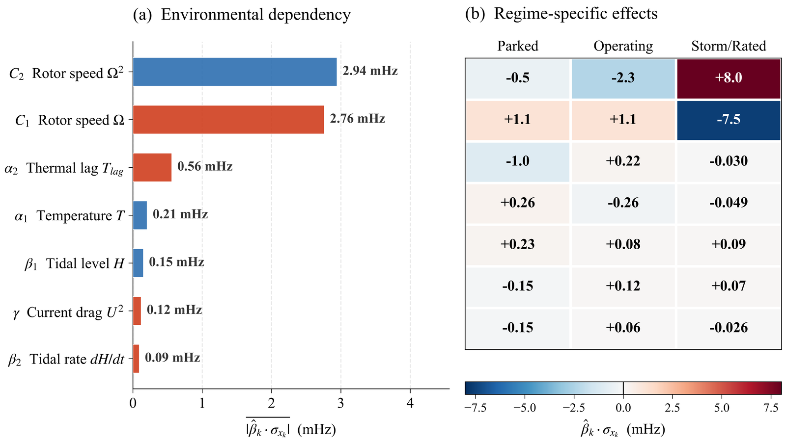
Figure 8: Environmental sensitivity of the first-mode frequency: (a) population-weighted mean absolute effect (\(\overline{|\hat{\beta}_k \cdot \sigma_{x_k}|}\), mHz) ranking the overall importance of each covariate, and (b) regime-specific signed effects revealing how each environmental coupling varies across Parked, Operating, and Storm/Rated states.

Table 6: Pooled Standardized OLS Regression on the Seven-Parameter EOV Model (\(n = 6{,}770\), \(R^2 = 0.205\)). Features ranked by \(|\hat{\beta}_{std}|\); the modest \(R^2\) reflects regime-mixing rather than weak environmental coupling. Significance: *** \(p < 0.001\); n.s. = not significant at \(\alpha = 0.05\).

Feature	Symbol	\(\hat{\beta}_{std}\)	\(p\)-value	Sig.	Physical Coeff.	Unit
Rotor speed \(\Omega\)	\(C_1\)	\(+1.333\)	\(< 0.001\)	***	\(+2.62 \times 10^{-3}\)	Hz/RPM
Rotor speed \(\Omega^2\)	\(C_2\)	\(-1.047\)	\(< 0.001\)	***	\(-2.05 \times 10^{-4}\)	Hz/RPM²
Thermal lag \(T_{\text{lag}}\)	\(\alpha_2\)	\(-0.294\)	\(< 0.001\)	***	\(-3.19 \times 10^{-4}\)	Hz/°C
Temperature \(T\)	\(\alpha_1\)	\(+0.220\)	\(< 0.001\)	***	\(+2.80 \times 10^{-4}\)	Hz/°C
Tidal level \(H\)	\(\beta_1\)	\(+0.076\)	\(< 0.001\)	***	\(+5.14 \times 10^{-4}\)	Hz/m
Current \(U^2\)	\(\gamma\)	\(+0.021\)	\(0.069\)	n.s.	\(+1.43 \times 10^{-3}\)	Hz/(m/s)²
Tidal rate \(\dot{H}\)	\(\beta_2\)	\(-0.016\)	\(0.142\)	n.s.	\(-3.30 \times 10^{-1}\)	Hz\(\cdot\)s/m

Efficacy of Normalization Method¶

The fitted coefficients (Table 7; Fig. 9) quantitatively confirm the mechanisms identified in Section 3.2. Tidal level \(\beta_1\) remains at order \(10^{-5}\)–\(10^{-4}\) Hz/m across all regimes, confirming structural decoupling of hydrodynamic effects. The dual-timescale thermal model, in which \(\alpha_1\) and \(\alpha_2\) carry opposing signs in Parked and Operating (consistent with competing surface-convective and bulk-conductive responses), contributes 15–20% additional variance beyond instantaneous ambient temperature. Both thermal coefficients collapse to order \(10^{-6}\) Hz/°C in Storm/Rated, where centrifugal terms dominate. The quadratic centrifugal term \(C_2\) is identifiable only in Storm/Rated (\(+3.89 \times 10^{-4}\) Hz/RPM²) where the RPM range permits separation from \(C_1\); regime intercepts increase from 240.8 (Parked) through 247.8 (Operating) to 277.4 mHz (Storm/Rated), independently corroborating centrifugal stiffening. The sign reversals (\(C_1\) from \(+8.10 \times 10^{-3}\) to \(-7.12 \times 10^{-3}\) Hz/RPM, \(\alpha_2\) from \(-1.13 \times 10^{-4}\) to \(+3.19 \times 10^{-5}\) Hz/°C across regimes) would be suppressed in a pooled model, confirming that regime splitting is essential.

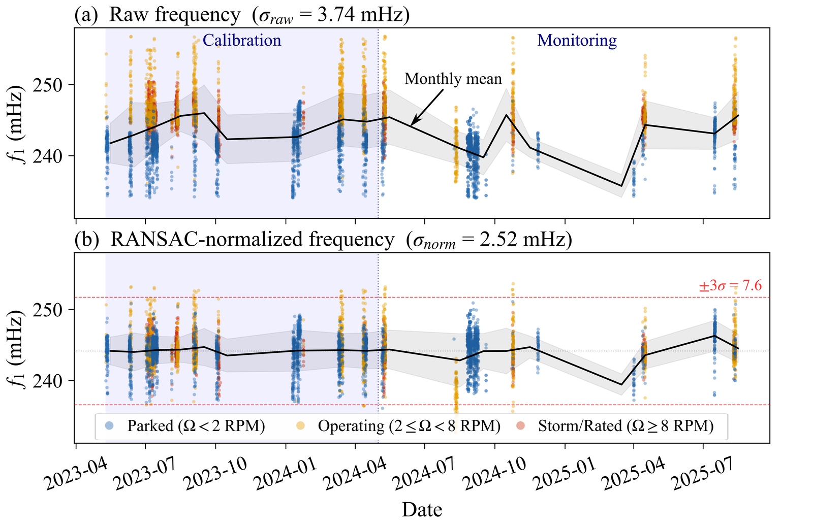
Figure 9: Regime-specific normalization effect: (a) raw first-mode frequency coloured by operational regime with monthly rolling statistics, and (b) RANSAC-normalized frequency with \(\pm 3\sigma\) control limits (red dotted horizontal line).

The pipeline progressively reduces first-mode scatter from \(\sigma_{raw} = 3.72\) mHz to \(\sigma_{resid} = 2.52\) mHz (32.3%, regression) and \(\sigma_{ewma} = 1.11\) mHz (70.1% total, EWMA span = 48; Fig. 9, Fig. 10). Regression absorbs systematic environmental coupling, collapsing the multimodal raw distribution (with regime-specific sub-populations near 240, 248, and 245 mHz) into a unimodal residual; EWMA then suppresses the residual high-frequency identification noise, a complementary spectral partition in which neither stage alone achieves the combined performance. The resulting near-Gaussian EWMA residual (Fig. 10 e, f) supports the \(3\sigma\) control-limit formulation in Section 3.4. RANSAC inlier consensus exceeded 97.8% in all regimes during the 12-month calibration, confirming that the seven-parameter model captures dominant deterministic mechanisms without overfitting.

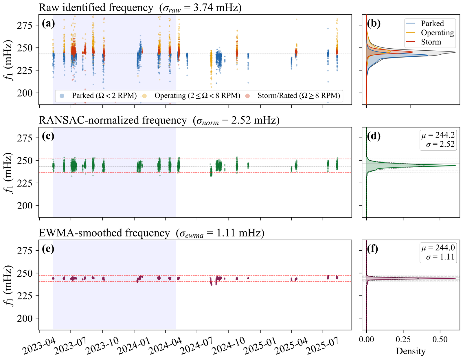
Figure 10: Three-stage normalization pipeline for the first-mode frequency over the 32-month monitoring field dataset. Left panels with calibration period indicated by the shaded region. Right panels: kernel density estimates with Gaussian overlays. (a, b) Raw identified frequency (\(\sigma_{raw} = 3.72\) mHz) showing regime-decomposed sub-populations; (c, d) RANSAC-normalized frequency (\(\sigma_{resid} = 2.52\) mHz); (e, f) EWMA residual (\(\sigma_{ewma} = 1.11\) mHz). Here, red dotted horizontal line represents \(\pm 3\sigma\) control limits

Table 7: Regime-Specific RANSAC Regression Coefficients (Mode 1, MAC \(> 0.85\), \(R^2 = 0.540\)). The intercept \(f_0^{(r)}\) represents the model-extrapolated frequency at zero regressor inputs; the Storm/Rated value (277.4 mHz) is an artefact of the uncentered RPM parameterization and should not be interpreted as a physical at-rest frequency.

Coefficient	Parked	Operating	Storm/Rated
\(f_0^{(r)}\) (mHz)	240.8	247.8	277.4
\(\beta_1\) (Hz/m)	\(+1.84 \times 10^{-4}\)	\(+6.10 \times 10^{-5}\)	\(+7.30 \times 10^{-5}\)
\(\beta_2\) (Hz\(\cdot\)s/m)	\(-8.36 \times 10^{-1}\)	\(+2.93 \times 10^{-1}\)	\(-1.37 \times 10^{-1}\)
\(\alpha_1\) (Hz/°C)	\(+2.82 \times 10^{-5}\)	\(-3.72 \times 10^{-5}\)	\(-7.32 \times 10^{-6}\)
\(\alpha_2\) (Hz/°C)	\(-1.13 \times 10^{-4}\)	\(+3.19 \times 10^{-5}\)	\(-4.56 \times 10^{-6}\)
\(\gamma\) (Hz/(m/s)²)	\(-1.30 \times 10^{-3}\)	\(+9.52 \times 10^{-4}\)	\(+5.32 \times 10^{-4}\)
\(C_1\) (Hz/RPM)	\(+8.10 \times 10^{-3}\)	\(+1.56 \times 10^{-3}\)	\(-7.12 \times 10^{-3}\)
\(C_2\) (Hz/RPM²)	\(-4.36 \times 10^{-3}\)	\(-2.53 \times 10^{-4}\)	\(+3.89 \times 10^{-4}\)

Field-Specific Sensitivity Matrix¶

We inject synthetic frequency-reduction vectors \(\Delta f = 0.12 \cdot (S/D)^{1.5} \cdot f_0\) into the 32-month field-derived residual and measure the detection probability \(P_d\) at each scour depth ratio \(S/D\) (Table 8). Because the residual encodes genuine seasonal, operational, and extreme-event variability, the resulting power curves reflect site conditions, not synthetic noise floors. Detection capability must be established through a stress test because no confirmed scour events occurred during the 32-month record (Section 4) according to our proposed framework. Three design levers govern sensitivity: (1) the EWMA smoothing window, which sets the noise floor \(\sigma_{cal}\); (2) the threshold multiplier, which trades sensitivity against false alarm rate; and (3) the persistence filter, which enforces geotechnical plausibility. The \(\sigma_{cal}\) values reported here (3.71 mHz at 8 h EWMA) exceed the RANSAC+EWMA residual (\(\sigma_{ewma} = 1.11\) mHz, Section 3.3) because the sensitivity matrix uses the baseline normalization residual—a deliberately conservative bound on system capability.

The EWMA window delivers the largest single gain: extending from 8 h to 48 h cuts \(\sigma_{cal}\) from 3.71 to 2.39 mHz (-35.6%), with diminishing returns beyond 24 h consistent with residual autocorrelation decay (Table 8). The 7-day persistence filter eliminates 100% of point-wise false alarms across all configurations tested, including \(2\sigma\) thresholds carrying unfiltered FAR of 6.6–7.9%. The physical basis for this filter is the pore pressure dissipation timescale of the 5.8 m clay stratum (\(c_v \approx 10^{-8}\)–\(10^{-7}\) m\(^2\)/s): no environmental exceedance persists beyond the drainage timescale, while genuine scour—an irreversible seabed loss—does. This geotechnical decoupling breaks the traditional FAR–sensitivity trade-off.

Table 8: Field-Specific Sensitivity Matrix. \(P_d\) is computed via scour-vector injection into the 32-month field-derived residual using the power law \(\Delta f/f_0 = 0.12 \cdot (S/D)^{1.5}\) [44] with \(f_0 = 243.3\) mHz and \(D = 8.0\) m. \(\sigma_{cal}\) is the field-calibrated noise floor computed over the 12-month calibration period (4,804 windows). FAR is the point-wise false alarm rate over the 20-month monitoring period (2,074 windows). Bold row indicates the optimal configuration.

EWMA	Threshold	Persistence	\(\sigma_{cal}\) (mHz)	Threshold (mHz)	FAR (%)	\(S/D\) at \(P_d = 90\%\)	\(S/D\) at \(P_d = 95\%\)
8 h	\(3\sigma\)	None	3.71	11.12	0.24	0.62	0.67
8 h	\(3\sigma\)	7-day	3.71	11.12	0.00	0.62	0.67
8 h	\(2\sigma\)	None	3.71	7.41	7.86	0.50	0.56
8 h	\(2\sigma\)	7-day	3.71	7.41	0.00	0.50	0.56
24 h	\(3\sigma\)	None	2.87	8.62	0.00	0.52	0.55
24 h	\(2\sigma\)	None	2.87	5.75	6.56	0.43	0.46
24 h	\(2\sigma\)	7-day	2.87	5.75	0.00	0.43	0.46
48 h	\(3\sigma\)	None	2.39	7.18	0.00	0.44	0.47
48 h	\(2\sigma\)	None	2.39	4.78	7.04	0.36	0.39
48 h	\(2\sigma\)	7-day	2.39	4.78	0.00	0.36	0.39

Combining all three levers quantifies the gain. The baseline configuration (8 h/\(3\sigma\)) reaches \(P_d = 95\%\) only at \(S/D = 0.67\); the 48 h/\(3\sigma\) setting shifts this to \(S/D = 0.47\)—71% of the total gain, from noise floor reduction alone—and adding the \(2\sigma\) threshold with 7-day persistence reaches the optimum at \(S/D = 0.39\), a 42% improvement over baseline (Fig. 11). At the \(0.24D\) deterministic limit, detection probability rises from 6.6% (baseline) to 66.5% (optimized), extending binary detection into a continuous probabilistic envelope. The persistence filter makes this threshold relaxation operationally viable: the 7-day window suppresses all 146 point-wise exceedances (out of 2,074 monitoring windows at 48 h/\(2\sigma\)) that would otherwise trigger unnecessary inspection campaigns.

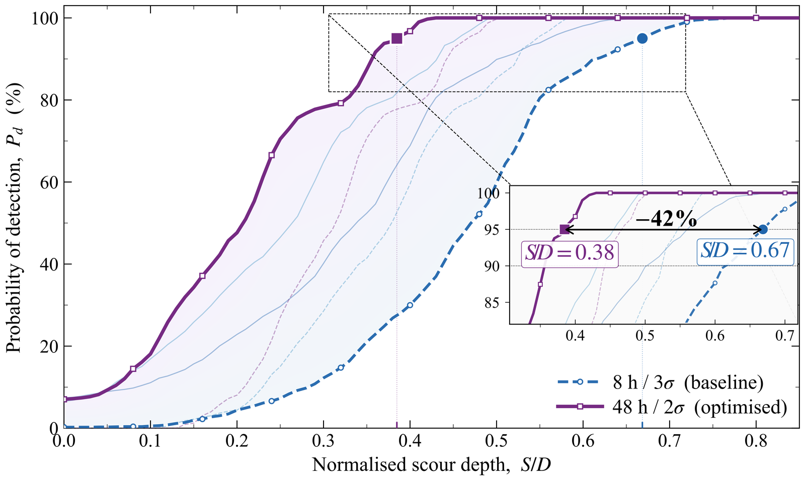
Figure 11: Detection power curves for six EWMA/threshold configurations via scour-vector injection into the 32-month field-calibrated noise floor. Thick lines: baseline (8 h/\(3\sigma\), dashed blue) and optimized (48 h/\(2\sigma\), solid purple) configurations. Square markers indicate \(P_d = 95\%\); the intermediate 48 h/\(3\sigma\) curve isolates noise floor reduction from threshold relaxation.

Discussion¶

The 32-month campaign confirms that EOV-induced frequency masking is predominantly deterministic and regime-dependent. The progressive scatter reduction (\(\sigma_{raw} = 3.72\) → \(\sigma_{resid} = 2.52\) → \(\sigma_{ewma} = 1.11\) mHz) yields a 2.2-fold improvement in equivalent scour sensitivity (from \(0.53D\) to \(0.24D\)), with noise floor reduction accounting for 71% of the total detection gain (Section 3.4). High-frequency identification scatter, rather than threshold design, is therefore the dominant barrier to scour detection.

Physical Interpretability¶

The regime-specific coefficients (Table 7) yield three engineering insights for tripod suction bucket foundations. First, a structural decoupling of hydrodynamic effects is observed. The tidal coefficient \(\beta_1\) remains at order \(10^{-5}\)–\(10^{-4}\) Hz/m across all regimes, an order of magnitude below the centrifugal terms (Fig. 8 a). This diverges from monopile typologies where tidal level dominates, and indicates that the EOV hierarchy for tripod foundations is centrifugally and thermally governed rather than mass-governed. SHM architectures based on monopile experience will consequently misallocate regressor capacity. Second, the dual-timescale thermal model captures the conductive lag through the steel-grout-soil system. The opposing signs of \(\alpha_1\) and \(\alpha_2\) in Parked and Operating (Table 7) are consistent with competing surface-convective and bulk-conductive responses, and both collapse to order \(10^{-6}\) Hz/°C in Storm/Rated where centrifugal terms dominate. Thermal models using only instantaneous ambient temperature will therefore underperform during seasonal transitions. Third, centrifugal stiffening is identifiable only in Storm/Rated, where the RPM range permits separation of the linear and quadratic terms; in Parked and Operating, narrow RPM spans produce collinear trade-off with negligible net contribution. The regime-split architecture is further necessitated by the layered stratigraphy, as each suction bucket penetrates all three strata and the relative contribution of each layer to rotational stiffness depends on the loading state, from small-strain clay response under parked conditions to cyclic pore pressure redistribution under storm loading. The resulting sign reversals across regimes produce the Simpson’s paradox identified in Section 3.2, where the pooled model grossly understates the resolved environmental coupling.

The RANSAC estimator provides a second layer of protection, namely robustness against the gross OMA identification failures (mode swapping, harmonic misidentification) characteristic of long-term autonomous monitoring. This constrained functional form cannot absorb path-dependent structural shifts into the environmental correction, unlike unconstrained projections such as PCA (Section 4.2). The post-regression residual is consequently dominated by stochastic identification scatter whose autocorrelation decays within the EWMA smoothing window, ensuring that temporal averaging operates on genuine noise rather than structured environmental trends. This spectral separation underlies the pipeline’s total scatter reduction (Section 3.3).

Benchmark Comparison with PCA-Based Method¶

A controlled full-pipeline comparison against PCA-based normalization, which is the most widely adopted method in the offshore wind SHM literature [27, 29], was conducted on an identical dataset and 12-month calibration protocol (MAC \(> 0.85\)). The PCA benchmark implements z-score standardization followed by PCA retaining 95% of environmental variance and OLS regression; with four input variables (tidal level, temperature, rotor speed, current velocity), all four principal components were retained, rendering dimensionality reduction inoperative and reducing the benchmark to OLS on standardized features.

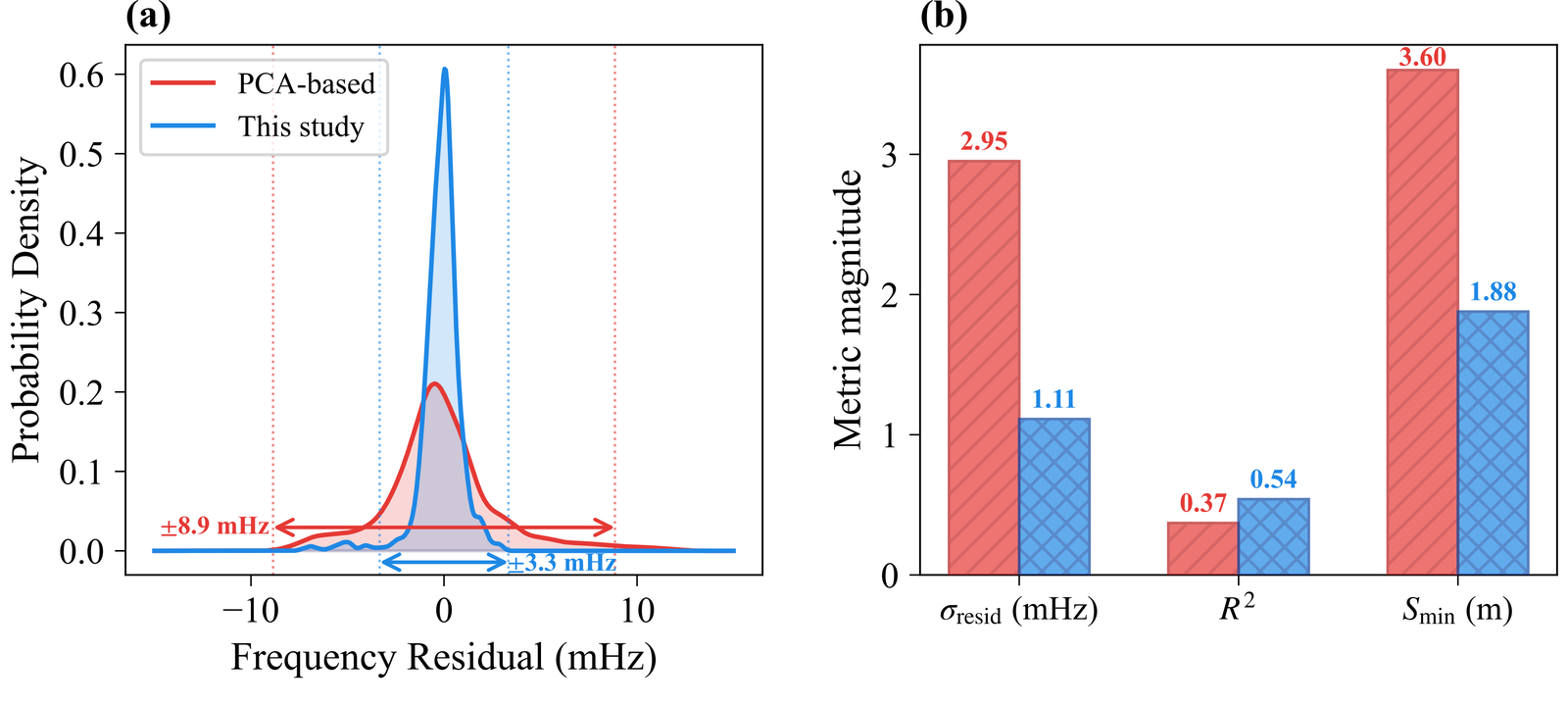
Figure 12: Benchmark comparison of PCA-based normalization and the proposed RANSAC+EWMA pipeline: (a) residual probability distributions with \(\pm 3\sigma\) detection envelopes, and (b) key performance metrics.

Fig. 12 and Table 9 summarise the full-pipeline comparison. At the regression stage alone, the RANSAC model already outperforms PCA-based method (\(\sigma_{resid} = 2.52\) mHz vs. 2.95 mHz; \(R^2 = 0.540\) vs. 0.370), confirming an intrinsic normalization advantage independent of any downstream signal conditioning. When the EWMA temporal smoothing is included, the performance gap widens substantially:

Table 9: Full-pipeline benchmark: PCA-based normalization vs. proposed RANSAC+EWMA framework. PCA-based values reflect the raw regression residual (no temporal smoothing); this study values include EWMA signal conditioning (span = 48 points, 8 h at 10-min cadence). The \(R^2\) is evaluated at the regression stage for both methods, as it measures the explained environmental variance prior to temporal averaging.

Metric	PCA-based	This study	Improvement
\(R^2\)	0.370	0.540	+45.8%
\(\sigma_{resid}\) (mHz)	2.95	1.11	-62.4%
\(S_{min}\)	3.60 m (\(0.45D\))	1.88 m (\(0.24D\))	-46.7%

A complementary sensitivity sweep over the PCA-hyperparameter space confirms that this advantage is not specific to the variance-maximising default of Table 9: grid-search over \(n_{\text{components}} \in \{2, 3, 5\}\) (exhaustive given the four-feature environmental basis) produces residual standard deviations of 9.27, 9.20, and 9.18 mHz respectively in the OLS-on-principal-components stage without EWMA smoothing, all substantially above the 2.52 mHz of raw RANSAC and the 1.11 mHz of RANSAC + EWMA; no choice of \(n_{\text{components}}\) brings the PCA family within reach of the proposed pipeline. The RANSAC model explains 54% of environmental variance (\(R^2 = 0.540\) vs. 0.370; +45.8%), with the improvement arising from regime separation eliminating cross-state residual structure and physics-informed features (tidal rate, 48-hour thermal lag, quadratic Campbell term) capturing nonlinear coupling that PCA’s linear set cannot represent. At the pre-EWMA stage, the RANSAC residual (\(\sigma = 2.52\) mHz) already shows a 14.6% reduction over PCA (\(\sigma = 2.95\) mHz); subsequent 8 h EWMA widens the gap to 62.4% (\(\sigma = 1.11\) vs. 2.95 mHz), with approximately one-quarter attributable to normalization and three-quarters to temporal averaging. The latter is enabled by the spectral separation engineered by the regression, which confines the residual to stochastic noise amenable to exponential smoothing. Beyond performance, PCA’s variance-maximizing projection constitutes a structural liability. Because it lacks any mechanism to enforce the state-function formulation (Eq. 3), PCA can absorb permanent scour-induced shifts during extreme events as latent correlations, normalizing away the damage signature [27, 29]. The constrained seven-parameter RANSAC model limits this damage leakage while providing coefficient-level diagnostic insight (regime-specific tidal sensitivities, thermal lag constants, and centrifugal stiffening rates) that is unavailable from black-box methods. The practical consequence is shown in Fig. 12 (a), where the PCA residual (\(3\sigma = \pm 8.85\) mHz) is 2.7 times wider than the proposed pipeline (\(3\sigma = \pm 3.33\) mHz), translating to equivalent scour thresholds of \(0.45D\) versus \(0.23D\) and a near-halving of minimum detectable depth.

Table 10 positions the present framework against the most directly relevant benchmarks in the offshore wind SHM literature. Because no prior field study on tripod suction bucket foundations reports both variance reduction and scour detection thresholds, the comparison includes the closest available field monitoring study and the data-driven normalization performance range from two independent reviews; the Scope column distinguishes field studies from review-level summaries.

Table 10: Field monitoring and normalization benchmarks in the offshore wind SHM literature. \(^\ddagger\)Range reported across the reviewed SHM literature; individual study results vary by method, structure, and application context. \(^*\)Total pipeline reduction including EWMA signal conditioning; regression-only reduction is 32.3%.

Study	Scope	Method	Variance Reduction	Detection Threshold
Devriendt et al. [16]; Weijtjens et al. [17]	Field; monopile	Automated OMA; regression normalization	—	—
Martinez-Luengo et al. [25]; Malekloo et al. [26]	Review; various	Data-driven (PCA, NN, SVR, GPR)	up to 70%\(^\ddagger\)	—
This study	Field; tripod	Regime-split RANSAC	70.1%\(^\)	\(0.24D\) (\(3\sigma\))

Regarding aforementioned comparison, three points warrant further discussion. First, the 70.1% total variance reduction exceeds the 50–70% range reported across the reviewed SHM literature for unconstrained data-driven methods [25, 26], while preserving coefficient-level physical interpretability and constraining the model’s capacity to absorb irreversible damage. Second, Devriendt et al. [16] and Weijtjens et al. [17] demonstrated automated OMA with regression-based normalization on a monopile, the closest methodological precedent, but reported neither quantitative variance reduction nor scour detection thresholds. The \(0.24D\) (\(3\sigma\)) and \(0.39D\) (\(P_d = 95\%\)) thresholds established here provide the first field-calibrated detection benchmarks for offshore wind foundations. Third, without environmental normalization the raw frequency scatter at this site yields an equivalent scour sensitivity of \(0.53D\) (\(S_{ESS,raw}\); Eq. 15), which the present pipeline reduces to \(0.24D\), a factor-of-2.2 improvement that confirms physics-informed EOV removal recovers detection capability otherwise masked by environmental scatter. For broader methodological context, Prendergast et al. [8] established the theoretical frequency–scour relationship for monopile foundations through numerical and laboratory analysis, providing the mechanistic basis for frequency-based detection, while Cross et al. [27] introduced cointegration for environmental trend removal in structural health monitoring; neither approach has been validated with field-based environmental normalization on offshore wind foundations.

Equivalent Scour Sensitivity and Detection of Change¶

Because the detection threshold is set as a multiple of the residual standard deviation, any reduction in \(\sigma\) lowers the smallest frequency shift distinguishable from noise. To translate this frequency-domain improvement into a physically interpretable scour metric, an Equivalent Scour Sensitivity (ESS) is defined by inverting the power-law relationship between frequency reduction and scour depth for tripod suction bucket foundations:

\[\frac{\Delta f}{f_0} = a \cdot \left(\frac{S}{D}\right)^b \quad \Rightarrow \quad S_{ESS} = D \cdot \left(\frac{\Delta f_{thresh}}{f_0 \cdot a}\right)^{1/b} \qquad(15)\]

where the coefficients \(a = 0.12\) and \(b = 1.5\), calibrated from centrifuge testing of tripod suction buckets in sand [44], are physically appropriate for the initial detection phase where the first \(0.31D\) of scour occurs within the surficial sand layer; at greater depths, erosion into the clay would modify both parameters. The ESS at three pipeline stages—\(S_{ESS,raw} = 0.53D\), \(S_{ESS,resid} = 0.40D\), \(S_{ESS,ewma} = 0.24D\)—confirms a 2.2-fold improvement.

The dual-panel control chart (Fig. 13) identified 55 discrete \(3\sigma\) exceedance events over 32 months, of which 54 were transient environmental forcing; one event (2023-09-08 to 2023-10-01) formally satisfied the 7-day persistence criterion but was diagnosed as a data sparsity artifact (positive residual inconsistent with scour, \(\theta_{max} = 0.046 < \theta_c = 0.047\)). The Tabular CUSUM registered 161 alarms, all recovering within 2–5 days. This provides stronger stationarity evidence than point-wise thresholds, because the CUSUM integrates successive observations and detects sustained shifts as small as \(1\sigma_{ewma}\) (\(\approx 0.11D\)). The zero-alarm record validates the three-stage pipeline against Type I errors across the full envelope of typhoon events, spring tide maxima, and emergency shutdowns, which is a prerequisite for autonomous deployment where false alarms carry direct operational cost.

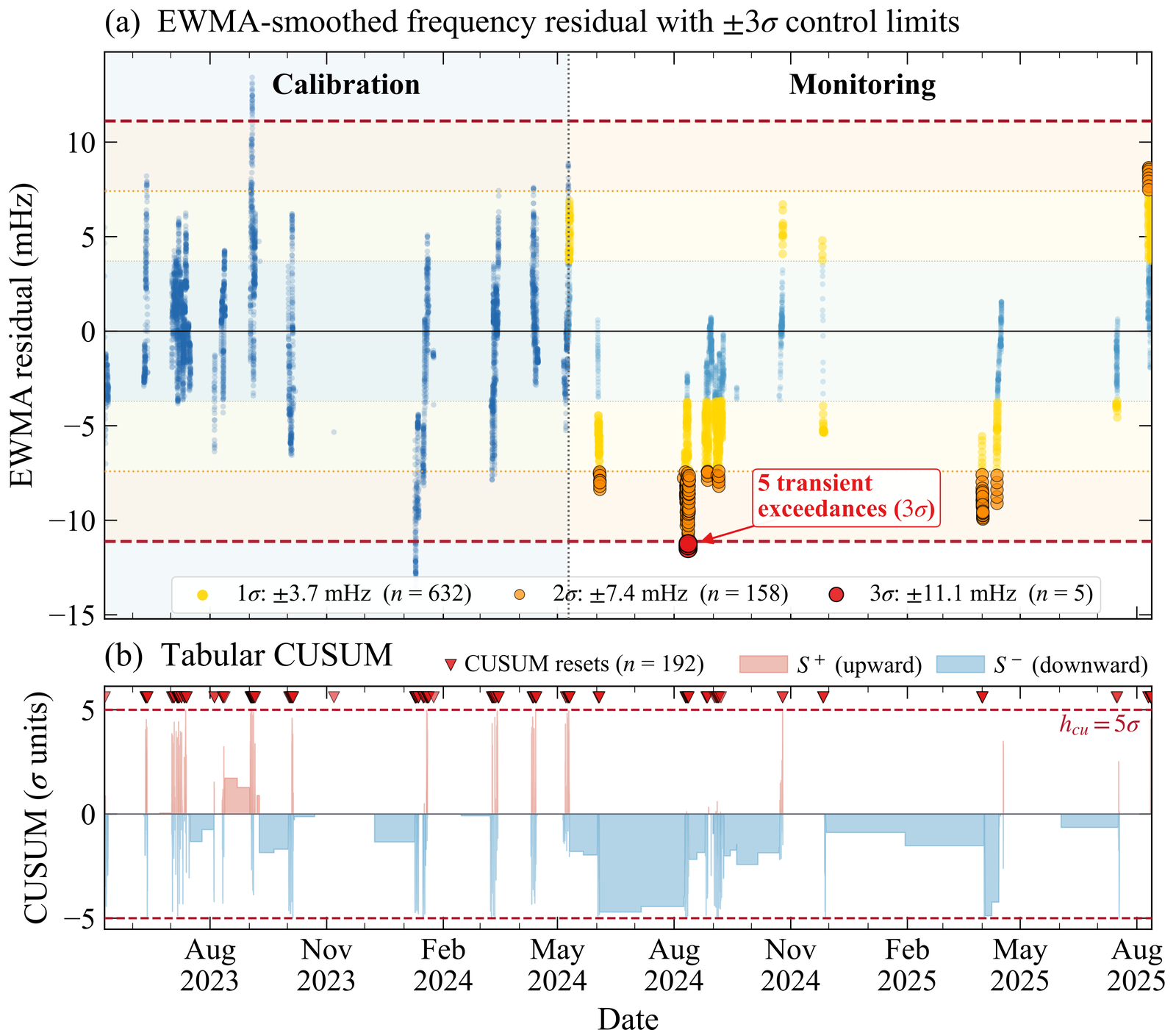
Figure 13: Dual-panel structural health control chart: (top) EWMA-smoothed frequency residual with \(\pm 3\sigma\) control limits, and (bottom) Tabular CUSUM upper and lower accumulators (\(S^+\), \(S^-\)) with the decision boundary \(h_{cu} = 5.0\sigma\). Transient alarm events are marked; all recovered within 2–5 days.

The Field-Specific Sensitivity Matrix (Table 8, Fig. 11) extends this to probabilistic detection: the optimized configuration shifts \(P_d = 95\%\) from \(0.67D\) to \(0.39D\), while the \(0.24D\) deterministic limit reaches \(P_d = 66.5\%\), enabling risk-based inspection scheduling at sub-threshold depths. The 7-day persistence filter makes this relaxation possible by exploiting the fundamental timescale separation between self-correcting environmental excursions and irreversible scour (\(c_v \approx 10^{-8}\)–\(10^{-7}\) m\(^2\)/s in the 5.8 m clay stratum) to decouple FAR from detection sensitivity.

Limitations¶

The framework is validated on a single 4.2 MW tripod at one site (sand/clay/sand stratigraphy); generalizability to other foundation types, soil conditions, turbine capacities, and wind climates remains unverified, and the regime boundaries (2, 8 RPM) are turbine-specific. The 32-month record validates Type I error performance; detection capability is characterized via synthetic injection rather than confirmed scour events. The additive damage assumption is conservative for storm-correlated scour, where damage leakage (Section 4.2) could reduce detection power. The sand-calibrated power-law coefficients (\(a = 0.12\), \(b = 1.5\)) [44] are appropriate for \(S \leq 0.31D\) (surficial sand layer); beyond 2.5 m, clay penetration would modify both parameters. The exponent \(b = 1.5\) produces diminishing sensitivity at incipient depths (\(S < 0.2D\)), establishing a fundamental single-mode resolution limit. The state-function formulation (Eq. 3) assumes memoryless environmental contributions; slow processes (soil consolidation, marine growth) may partially violate this but produce gradual drift distinguishable from step-like scour. Within-regime linearity does not capture nonlinear cross-coupling between covariates. The MAC gate retains 30.4% of windows, creating temporal blind spots, and the merged FA/SS modes limit directional diagnosis; submerged instrumentation could improve both yield and sensitivity.

The sensitivity matrix uses the conservative baseline residual (\(\sigma_{cal} = 3.71\) mHz) rather than the RANSAC residual (\(\sigma_{ewma} = 1.11\) mHz), ensuring detection limits represent a lower bound. The \(3\sigma\) threshold assumes approximate Gaussianity; departures would modify the empirical FAR. The 20-month monitoring period yields \(n \approx 50\)–87 independent 7-day evaluation windows; applying the rule of three gives an upper 95% Clopper-Pearson bound of 3–6% on per-event false alarm probability; multi-turbine deployment would narrow this bound. The 48 h EWMA introduces ~2-day latency, acceptable for clay-governed scour progression but not for sudden damage (vessel impact, extreme waves), where the 8 h baseline or direct acceleration-based detection is appropriate. The persistence filter’s universality is tied to this site’s clay drainage timescale; transferability to sites lacking a comparable low-permeability stratum requires validation. The modular design of the architecture can accommodate multi-site data as they become available, though site-specific recalibration will be required.

Limitations of synthetic damage injection¶

Detection performance is characterised through synthetic damage injection because no confirmed scour events occurred over the 32-month record. Three qualifiers on this approach deserve explicit disclosure. First, the injected frequency shifts are linear super-positions on top of the existing residual record and therefore do not reproduce the mild nonlinear cross-coupling that real scour would induce via strain-amplitude-dependent soil stiffness and via the tidal-current – scour-geometry feedback loop; the linear-injection residual distribution is a conservative approximation that tends to overstate detection capability for soft events and understate it for stiff-regime events, and the direction of the bias is not uniform across the \(S/D\) range. Second, the injection magnitude follows the centrifuge-calibrated power law \(\Delta f/f_0 = -0.12 \cdot (S/D)^{1.5}\) of the Kim companion [44] rather than the clay-prototype Winkler-calibrated power law \(\Delta f/f_0 = -0.167 \cdot (S/D)^{1.47}\) of the OE-D-26-00984 companion paper; the two coefficients differ because of the clay-vs-sand constitutive residual documented in OE-D-26-00984, so the reported detection probabilities should be read as centrifuge-calibrated sand-equivalent injection rather than as site-specific clay-calibrated injection. The choice of the more conservative (smaller \(|a|\)) coefficient here is deliberate: it produces a lower-bound detection probability at each \(S/D\), so the zero-false-alarm + Pd\(\geq 90\%\) at \(S/D = 0.62\) result is a lower bound rather than a best-case estimate. Third, real scour evolves over timescales of weeks to months and is typically spatially asymmetric around a multi-footing foundation, whereas the synthetic injection applies a single instantaneous symmetric shift to the full parked-state residual population. The resulting detection curves therefore bound the performance of the pipeline on geometrically symmetric scour; asymmetric scour would break the rotational-stiffness symmetry that the current implementation assumes and would require the per-bucket detection extension reserved for future work.

Conclusion¶

This study presents a 32-month field validation of the physics-informed Double-Filter framework for vibration-based scour detection, applied to a 4.2 MW tripod-supported offshore wind turbine with suction bucket foundations in the West Sea of Korea (May 2023–December 2025). The framework couples regime-split RANSAC regression with a three-stage detection pipeline that enforces a state-function distinction between reversible environmental effects and irreversible structural degradation. It achieved a zero-false-alarm record across 22,616 synchronized ten-minute windows spanning the full envelope of seasonal, storm, and operational variability, with 6,878 high-quality estimates (MAC \(> 0.85\)) forming the basis for environmental normalization and detection sensitivity characterization.

The primary findings are summarized below.

The pipeline achieved a 70.1% total scatter reduction (\(\sigma_{raw} = 3.72\) → \(\sigma_{ewma} = 1.11\) mHz), with the regression stage explaining 54.0% of environmental variance, a 45.8% improvement over PCA-based normalization on the same dataset.
The seven-parameter physics-constrained model enforces environmental reversibility by construction, limiting the capacity to absorb irreversible structural shifts. The 32-month zero-alarm record with bounded CUSUM accumulators provides indirect validation that no latent structural trend was absorbed into the environmental correction.
The Field-Specific Sensitivity Matrix, evaluated against the 32-month empirical noise floor, established \(P_d = 95\%\) at \(0.39D\) (3.12 m) under the optimized configuration and a deterministic \(3\sigma\) sensitivity of \(0.24D\), a 2.2-fold improvement over raw scatter.
The 7-day persistence filter and Shields gate eliminated 100% of environmental false alarms over 2,074 monitoring windows, including 146 exceedances at \(2\sigma\)/48 h EWMA. This result demonstrates that geotechnical timescale separation decouples FAR from detection sensitivity.
Tripod suction buckets exhibit negligible tidal sensitivity (\(\beta_1 \sim 10^{-5}\)–\(10^{-4}\) Hz/m), diverging from monopile typologies. The 48-hour thermal lag explained 15–20% additional variance, confirming that thermal normalization of massive offshore substructures requires explicit treatment of the conductive lag through the steel-grout-soil system.

The detection limits of the proposed Double-Filter framework are anchored in a 32-month empirical noise floor rather than idealized simulations. The site’s layered stratigraphy simultaneously defines both the valid detection range (\(S \le 0.31D\) in surficial sand) and the persistence filter’s drainage timescale (intermediate clay). These results establish a validated framework, transferable in functional form though requiring site-specific recalibration, for future multi-site deployment and integration with model-based digital twin paradigms [45] for multi-modal probabilistic data fusion.

Data Availability¶

The raw structural vibration and SCADA data were collected under a Korea Institute of Energy Research (KIER) monitoring program and are subject to institutional confidentiality agreements. Processed modal parameter datasets, environmental state vectors, and computational routines are available from the corresponding author upon reasonable request.

Acknowledgments¶

This work was supported by Korea Electric Power Corporation (Grant No. R23XO05-01), the National Research Foundation of Korea (NRF) grant funded by the Korea government (MSIT) (Grant No. RS-2022-NR070302), the Korea Institute of Energy Technology Evaluation and Planning(KETEP) and the Ministry of Trade, Industry & Energy(MOTIE) of the Republic of Korea (NO. RS-2025-02318006), and the Korea Institute of Marine Science & Technology Promotion(KIMST) funded by the Ministry of Oceans and Fisheries(RS-2025-02304428). The authors gratefully acknowledge the Korea Institute of Energy Research (KIER) for granting access to the long-term field monitoring data that enabled the experimental validation presented in this study.

CRediT Author Contributions¶

Kyeong-Sun Kim: Conceptualization, Methodology, Software, Validation, Formal analysis, Investigation, Writing – Original Draft, Visualization. Seongho Hong: Software, Validation. Gwang-Se Lee: Resources, Data Curation. Moo-Sung Ryu: Funding acquisition, Project administration. Sung-Ryul Kim: Conceptualization, Supervision, Project administration, Funding acquisition, Writing – Review & Editing.

Declaration of Competing Interests¶

The authors declare no known competing financial interests or personal relationships that could have appeared to influence the work reported in this paper.

References¶

\[1\] GWEC, Global offshore wind report 2024, *Global Wind Energy Council* (2024)

\[2\] Arany, L., Bhattacharya, S., Macdonald, J., Hogan, S.J., Design of monopiles for offshore wind turbines in 10 steps, *Soil Dynamics and Earthquake Engineering* 92 (2017) 126–152. [doi.org/10.1016/j.soildyn.2016.09.024](https://doi.org/10.1016/j.soildyn.2016.09.024)

\[3\] Byrne, B.W., Houlsby, G.T., Helical piles: An innovative foundation design option for offshore wind turbines, *Philosophical Transactions of the Royal Society A* 373 (2015) 20140081. [doi.org/10.1098/rsta.2014.0081](https://doi.org/10.1098/rsta.2014.0081)

\[4\] Melville, B.W., Coleman, S.E., Bridge scour, Water Resources Publications, Colorado, USA, 2000

\[5\] Prendergast, L.J., Reale, C., Gavin, K., Probabilistic examination of the change in eigenfrequencies of an offshore wind turbine under progressive scour incorporating soil spatial variability, *Marine Structures* 57 (2018) 87–104. [doi.org/10.1016/j.marstruc.2017.09.009](https://doi.org/10.1016/j.marstruc.2017.09.009)

\[6\] Sørensen, S.P.H., Ibsen, L.B., Assessment of foundation design for offshore monopiles unprotected against scour, *Ocean Engineering* 63 (2013) 17–25. [doi.org/10.1016/j.oceaneng.2013.01.016](https://doi.org/10.1016/j.oceaneng.2013.01.016)

\[7\] Prendergast, L.J., Hester, D., Gavin, K., O’Sullivan, J.J., An investigation of the changes in the natural frequency of a pile affected by scour, *Journal of Sound and Vibration* 332 (2013) 6685–6702. [doi.org/10.1016/j.jsv.2013.08.020](https://doi.org/10.1016/j.jsv.2013.08.020)

\[8\] Prendergast, L.J., Gavin, K., Doherty, P., An investigation into the effect of scour on the natural frequency of an offshore wind turbine, *Ocean Engineering* 101 (2015) 1–11. [doi.org/10.1016/j.oceaneng.2015.04.017](https://doi.org/10.1016/j.oceaneng.2015.04.017)

\[9\] Kim, S.-R., Hung, L.C., Oh, M., Group effect on bearing capacities of tripod bucket foundations in undrained clay, *Ocean Engineering* 79 (2014) 1–9. [doi.org/10.1016/j.oceaneng.2013.12.017](https://doi.org/10.1016/j.oceaneng.2013.12.017)

\[10\] Hung, L.C., Kim, S.-R., Evaluation of combined horizontal-moment bearing capacities of tripod bucket foundations in undrained clay, *Ocean Engineering* 85 (2014) 100–109. [doi.org/10.1016/j.oceaneng.2014.04.025](https://doi.org/10.1016/j.oceaneng.2014.04.025)

\[11\] Tran, N.X., Hung, L.C., Kim, S.-R., Evaluation of horizontal and moment bearing capacities of tripod bucket foundations in sand, *Ocean Engineering* 140 (2017) 209–221. [doi.org/10.1016/j.oceaneng.2017.05.030](https://doi.org/10.1016/j.oceaneng.2017.05.030)

\[12\] Doherty, J.P., Deeks, A.J., Elastic response of circular footings embedded in a non-homogeneous half-space, *Géotechnique* 53 (2003) 703–714. [doi.org/10.1680/geot.2003.53.8.703](https://doi.org/10.1680/geot.2003.53.8.703)

\[13\] Hardin, B.O., The nature of stress-strain behavior for soils, *Earthquake Engineering and Soil Dynamics — Proceedings of the ASCE Geotechnical Engineering Division Specialty Conference* 1 (1978) 3–90

\[14\] Seo, Y.-H., Ryu, M.S., Oh, K.-Y., Dynamic characteristics of an offshore wind turbine with tripod suction buckets via full-scale testing, *Complexity* 2020 (2020) 3079308. [doi.org/10.1155/2020/3079308](https://doi.org/10.1155/2020/3079308)

\[15\] Jeong, Y.H., Ko, K.W., Kim, D.S., Kim, J.H., Studies on cyclic behavior of tripod suction bucket foundation system supporting offshore wind turbine using centrifuge model test, *Wind Energy* 24 (2021) 515–529. [doi.org/10.1002/we.2586](https://doi.org/10.1002/we.2586)

\[16\] Devriendt, C., Magalhães, F., Weijtjens, W., Sitter, G. de, Cunha, Á., Guillaume, P., Structural health monitoring of offshore wind turbines using automated operational modal analysis, *Structural Health Monitoring* 13 (2014) 644–659. [doi.org/10.1177/1475921714556568](https://doi.org/10.1177/1475921714556568)

\[17\] Weijtjens, W., Verbelen, T., De Sitter, G., Devriendt, C., Foundation structural health monitoring of an offshore wind turbine—a full-scale case study, *Structural Health Monitoring* 15 (2016) 389–402. [doi.org/10.1177/1475921715586624](https://doi.org/10.1177/1475921715586624)

\[18\] Tang, D., Zhao, M., Real-time monitoring system for scour around monopile foundation of offshore wind turbine, *Journal of Civil Structural Health Monitoring* (2021). [doi.org/10.1007/s13349-020-00467-4](https://doi.org/10.1007/s13349-020-00467-4)

\[19\] Weil, M., Sastre Jurado, C., Chaar, M., Winkler, K., Weijtjens, W., Devriendt, C., Quantifiable scour detection for offshore wind turbines using resonance frequency monitoring and a digital twin, *Structural Health Monitoring (Proc.)* (2023). [doi.org/10.12783/shm2023/37048](https://doi.org/10.12783/shm2023/37048)

\[20\] Harte, M., Basu, B., Nielsen, S.R.K., Dynamic analysis of wind turbines including soil-structure interaction, *Engineering Structures* 45 (2012) 509–518. [doi.org/10.1016/j.engstruct.2012.06.041](https://doi.org/10.1016/j.engstruct.2012.06.041)

\[21\] Damgaard, M., Andersen, L.V., Ibsen, L.B., Computationally efficient modelling of dynamic soil–structure interaction of offshore wind turbines on gravity footings, *Renewable Energy* 68 (2014) 289–303. [doi.org/10.1016/j.renene.2014.02.008](https://doi.org/10.1016/j.renene.2014.02.008)

\[22\] Damgaard, M., Bayat, M., Andersen, L.V., Ibsen, L.B., Assessment of the dynamic behaviour of saturated soil subjected to cyclic loading from offshore monopile wind turbine foundations, *Computers and Geotechnics* 61 (2014) 116–126. [doi.org/10.1016/j.compgeo.2014.05.008](https://doi.org/10.1016/j.compgeo.2014.05.008)

\[23\] Damgaard, M., Andersen, L.V., Ibsen, L.B., Dynamic response sensitivity of an offshore wind turbine for varying subsoil conditions, *Ocean Engineering* 101 (2015) 227–234. [doi.org/10.1016/j.oceaneng.2015.04.039](https://doi.org/10.1016/j.oceaneng.2015.04.039)

\[24\] Avendaño-Valencia, L.D., Chatzi, E.N., Tcherniak, D., Gaussian process models for mitigation of operational variability in the structural health monitoring of wind turbines, *Mechanical Systems and Signal Processing* 142 (2020) 106686. [doi.org/10.1016/j.ymssp.2020.106686](https://doi.org/10.1016/j.ymssp.2020.106686)

\[25\] Martinez-Luengo, M., Kolios, A., Wang, L., Structural health monitoring of offshore wind turbines: A review through the statistical pattern recognition paradigm, *Renewable and Sustainable Energy Reviews* 64 (2016) 91–105. [doi.org/10.1016/j.rser.2016.05.085](https://doi.org/10.1016/j.rser.2016.05.085)

\[26\] Malekloo, A., Ozer, E., AlHamaydeh, M., Girolami, M., Machine learning and structural health monitoring overview with emerging technology and high-dimensional data source highlights, *Structural Health Monitoring* 21 (2022) 1906–1955. [doi.org/10.1177/14759217211036880](https://doi.org/10.1177/14759217211036880)

\[27\] Cross, E.J., Worden, K., Chen, Q., Cointegration: A novel approach for the removal of environmental trends in structural health monitoring data, *Proceedings of the Royal Society A* 467 (2011) 2712–2732. [doi.org/10.1098/rspa.2011.0023](https://doi.org/10.1098/rspa.2011.0023)

\[28\] Cross, E.J., Koo, K.Y., Brownjohn, J.M.W., Worden, K., Long-term monitoring and data analysis of the Tamar Bridge, *Mechanical Systems and Signal Processing* 35 (2013) 16–34. [doi.org/10.1016/j.ymssp.2012.08.026](https://doi.org/10.1016/j.ymssp.2012.08.026)

\[29\] Worden, K., Cross, E.J., On switching response surface models, with applications to the structural health monitoring of bridges, *Mechanical Systems and Signal Processing* 98 (2018) 139–156. [doi.org/10.1016/j.ymssp.2017.04.022](https://doi.org/10.1016/j.ymssp.2017.04.022)

\[30\] Karniadakis, G.E., Kevrekidis, I.G., Lu, L., Perdikaris, P., Wang, S., Yang, L., Physics-informed machine learning, *Nature Reviews Physics* 3 (2021) 422–440. [doi.org/10.1038/s42254-021-00314-5](https://doi.org/10.1038/s42254-021-00314-5)

\[31\] Rogers, T.J., Worden, K., Cross, E.J., On the application of Gaussian process latent force models for joint input-state-parameter estimation: With a view to Bayesian operational identification, *Mechanical Systems and Signal Processing* 140 (2020) 106580. [doi.org/10.1016/j.ymssp.2019.106580](https://doi.org/10.1016/j.ymssp.2019.106580)

\[32\] Jalbi, S., Bhattacharya, S., Closed form solution for the first natural frequency of offshore wind turbine jackets supported on multiple foundations incorporating soil-structure interaction, *Soil Dynamics and Earthquake Engineering* 113 (2018) 593–613. [doi.org/10.1016/j.soildyn.2018.06.011](https://doi.org/10.1016/j.soildyn.2018.06.011)

\[33\] Houlsby, G.T., Ibsen, L.B., Byrne, B.W., Suction caissons for wind turbines, *Frontiers in Offshore Geotechnics: ISFOG 2005* (2005) 75–93

\[34\] Suryasentana, S.K., Burd, H.J., Byrne, B.W., Shonberg, A., A systematic framework for formulating convex failure envelopes in multiple loading dimensions, *Géotechnique* 70 (2020) 343–353. [doi.org/10.1680/jgeot.18.p.251](https://doi.org/10.1680/jgeot.18.p.251)

\[35\] Figueiredo, E., Park, G., Farrar, C.R., Worden, K., Figueiras, J., Machine learning algorithms for damage detection under operational and environmental variability, *Structural Health Monitoring* 10 (2010) 559–572. [doi.org/10.1177/1475921710388971](https://doi.org/10.1177/1475921710388971)

\[36\] Ryu, M.-S., Lee, J.-S., Kwag, D., Seo, Y.-H., Verification of tripod suction pile applicability through dynamic characteristic analysis of offshore wind turbine at each installation stage, *Journal of the Korean Wind Energy Association* 10 (2019) 12–21

\[37\] Ryu, M.-S., Kim, S.-R., Cho, D.-H., Kang, J.-G., Innovative single-day installation vessel for offshore wind turbines, *Energies* 15 (2022) 3914. [doi.org/10.3390/en15113914](https://doi.org/10.3390/en15113914)

\[38\] DNV, Offshore soil mechanics and geotechnical engineering, DNV, 2021

\[39\] Virtanen, P., Gommers, R., Oliphant, T.E., others, SciPy 1.0: Fundamental algorithms for scientific computing in Python, *Nature Methods* 17 (2020) 261–272. [doi.org/10.1038/s41592-019-0686-2](https://doi.org/10.1038/s41592-019-0686-2)

\[40\] Peeters, B., De Roeck, G., Reference-based stochastic subspace identification for output-only modal analysis, *Mechanical Systems and Signal Processing* 13 (1999) 855–878. [doi.org/10.1006/mssp.1999.1249](https://doi.org/10.1006/mssp.1999.1249)

\[41\] Reynders, E., System identification methods for (operational) modal analysis: Review and comparison, *Archives of Computational Methods in Engineering* 19 (2012) 51–124. [doi.org/10.1007/s11831-012-9069-x](https://doi.org/10.1007/s11831-012-9069-x)

\[42\] Huber, P.J., Robust estimation of a location parameter, *Annals of Mathematical Statistics* 35 (1964) 73–101. [doi.org/10.1214/aoms/1177703732](https://doi.org/10.1214/aoms/1177703732)

\[43\] Soulsby, R., Dynamics of marine sands: A manual for practical applications, Thomas Telford, London, 1997

\[44\] Kim, K.-S., Oh, S.-W., Kim, B.-S., Kim, S.-R., Investigating scour impacts on natural frequency changes and sensitivity in offshore wind turbine with tripod suction bucket foundations in sand, *Ocean Engineering* 342 (2025) 123084. [doi.org/10.1016/j.oceaneng.2025.123084](https://doi.org/10.1016/j.oceaneng.2025.123084)

\[45\] Song, M., Moaveni, B., Ebrahimian, H., Hines, E.M., Bajric, A., Joint parameter-input estimation for digital twinning of the Block Island wind turbine using output-only measurements, *Mechanical Systems and Signal Processing* 198 (2023) 110425. [doi.org/10.1016/j.ymssp.2023.110425](https://doi.org/10.1016/j.ymssp.2023.110425)