Author's accepted manuscript
This page is the author's accepted manuscript (AAM) of a paper in preparation for Computers and Geotechnics. Status: drafting; target submission 2026-06-15. The text below is the post-peer-review revision; the publisher's typeset version (the version of record) is authoritative.
Version of record: DOI will be added here once the publisher posts the typeset version.
Shared under CC BY-NC-ND 4.0, in accordance with the publisher's author-sharing policy.
Summary
Full title
What Works and What Doesn't for Tripod Foundation Scour Detection: A Buckingham-Pi Feature Ranking with Centrifuge-to-Field Transfer.
One-sentence headline
Five dimensionless monitoring features derived via Buckingham-Pi analysis and ranked by bootstrap confidence intervals on a labelled 22-test centrifuge programme — with the strain–acceleration coherence feature transferring to 32 months of Gunsan field data to produce a measured +55.8 % shift at the only scour event in the record.
Context
Hundreds of vibration features have been proposed for offshore-foundation scour detection: frequency, damping, mode shape, MAC, strain-acceleration coupling, coherence, fixity ratios. No study has systematically ranked them on a labelled dataset where every feature sees the same scour stages. For tripod buckets the need is acute: frequency — the default feature — shows only 5 % shift at \(S/D = 0.6\), barely above the EOV floor. If another feature has higher signal-to-EOV ratio, it should be the primary monitoring channel — but only a head-to-head benchmark can prove it.
Research question
Among the combinatorial space of vibration-derived features, which subset is simultaneously sensitive to scour and insensitive to environmental variability across different soil conditions, and which one transfers from centrifuge model to operational field scale without per-site recalibration?
Approach
Five features constructed from Buckingham-Pi dimensional analysis so that each is scale-invariant between model (centrifuge) and prototype (field): normalised frequency shift, dimensionless damping ratio, MAC, strain-fixity ratio, and mid-elevation strain–acceleration coherence. Each feature is computed on all 22 centrifuge tests across 5 soil series (T1–T5) at every scour stage, producing a labelled ranking dataset. Bootstrap 95 % confidence intervals quantify feature reliability. The top-ranked feature is then computed on the 32-month Gunsan field record as a cross-domain transfer test.
Gap the paper closes
- Defensive. No systematic feature-ranking study has been conducted on a labelled tripod-bucket scour dataset.
- Offensive. Hundreds of feature proposals have appeared in the SHM literature with no mutual benchmarking; frequency has been the default only because it was first, not because it was best.
- Constructive. Produces the feature ranking that V uses as its primary detection channel and that A weighs in its value-of-information analysis.
Key literature anchors
- Buckingham (1914) — the Pi theorem.
- Worden et al. (2015) — novelty detection on the Z-24 bridge; canonical SHM benchmark paper.
- Li et al. (2020) — scour-frequency sensitivity across scour extents.
- Kariyawasam & Middleton (2020) — mode-shape vs frequency sensitivity for bridge piers.
- Jalbi & Bhattacharya (2018) — multi-footing frequency insensitivity.
Headline findings
- Strain–acceleration coherence ranks #1: sign-consistent across all five soil series, Cohen's d = −1.65 between pre- and post-scour distributions.
- Strain fixity ratio fails: inconsistent sign across soils, not a reliable standalone feature.
- Frequency shift ranks #3: usable but noisier than coherence on tripod geometry.
- Cross-domain transfer: coherence feature on 32-month Gunsan record shows measured +55.8 % shift at the only scour event observed — first quantitative confirmation of centrifuge-to-field transfer via Buckingham-Pi normalisation.
- π₆ (a candidate feature derived from the theorem) is a null result: included for honest reporting.
Limitations
- Feature space is not exhaustive — wavelet-based features, higher-order statistics, and learning-based features are out of scope.
- Labelled dataset is centrifuge-only; field transfer is one event.
- Bootstrap confidence intervals assume iid test samples; the 22 centrifuge tests have known inter-test correlation through shared model bucket geometry.
Portfolio flow
- Consumes: J1 / J3 centrifuge data; Op3 pipeline for scale-invariance check.
- Produces: feature ranking → V primary detection channel; feature VoI → A Bayesian fusion weights.
Status
Draft complete. Target submission to Computers and Geotechnics 2026-06-15.
Introduction
Scour detection in offshore wind turbine foundations has relied on tracking the first natural frequency, which decreases as soil erosion reduces the lateral restraint on the foundation1. For monopile foundations, frequency reductions of 5 to 12% per pile diameter of scour have been documented under field conditions2, and methods for separating scour-induced shifts from environmental and operational variability (EOV, the collective influence of temperature, tidal level, wind speed, and turbine operating state on structural response) are mature, ranging from regression-based normalization3 to tree-based machine learning4. Tripod suction bucket (TSB) foundations respond differently. Because three separate buckets share the applied loads, stiffness loss at one bucket is partially compensated by the remaining two, and the resulting frequency change is suppressed. Centrifuge experiments on a 1:70 scale model of a 4.2 MW prototype at 70g gravitational acceleration produced frequency reductions of only 0.85 to 5.3% at scour depths up to 0.6 bucket diameters5,6, roughly two to five times less than monopile values at comparable normalized depths.7 reported an even smaller effect in a numerical study of a tripod pile foundation, describing the frequency sensitivity as “minor.” No scour monitoring framework has been developed for TSB foundations, and the question of whether any vibration-based feature can reliably detect scour in these systems remains open.
The problem can be framed within the statistical pattern recognition paradigm for structural health monitoring, as formalised by8 and9. In this paradigm, monitoring proceeds through four stages: operational evaluation, data acquisition, feature extraction, and statistical modelling for feature discrimination. The choice of damage-sensitive feature is widely recognised as the most consequential decision in the entire pipeline10, because a feature that is insensitive to the damage mechanism of interest cannot be compensated by more sophisticated classification algorithms. For scour in TSB foundations, this choice is nontrivial: the conventional feature (first natural frequency) is weakly sensitive due to the multi-footing load redistribution described above, and no alternative has been systematically evaluated. The work reported here operates within this paradigm, with Buckingham Pi dimensional analysis providing the feature extraction and normalization, and cosine-similarity-based nearest-centroid classification providing the statistical modelling.
A related challenge is the absence of labeled field data. Centrifuge experiments provide scour depth labels at each test stage, but the measured quantities differ from field values by the centrifuge scaling factor N = 70 in frequency and acceleration. Field monitoring captures authentic environmental conditions but provides no independent scour measurement against which to calibrate a detector. This labeled-source, unlabeled-target structure is a domain transfer problem.11 addressed a version of it for monopiles by using a finite-element digital twin to predict frequency sensitivity, but digital twins require model calibration and cannot reproduce the nonlinear soil behaviour that centrifuge models inherit from physical scaling. Buckingham Pi dimensional analysis, which underpins centrifuge scaling itself12,13, offers an alternative: if features are expressed as non-dimensional ratios, the scaling factor cancels, and centrifuge and field values become directly comparable without statistical domain adaptation. Although dimensional analysis has been applied extensively to scale physical quantities in centrifuge modelling, it has not been applied to construct transferable damage-sensitive features for structural health monitoring.
The strain distribution along the tower provides scour information that frequency alone does not capture. When scour lowers the effective fixity point, the bending moment distribution shifts, altering both the amplitude ratios and the spectral coherence between strain channels at different elevations. The strain fixity ratio (bottom-to-top amplitude ratio) is an intuitive candidate because it is already dimensionless and independent of excitation amplitude.6 observed in centrifuge tests that at a scour depth of 0.58 bucket diameters in loose saturated sand, the bottom strain reversed from positive to negative while the frequency decreased by only 2.6%, indicating a bending-to-tilting transition that frequency monitoring could not detect. However, no study has systematically evaluated which strain-derived features actually separate healthy from scoured states across multiple soil conditions.14 and15 applied multi-feature statistical approaches (principal component analysis and Naive Bayes classification, respectively) to structural damage detection, but neither included strain-acceleration cross-spectral features nor addressed multi-footing foundations. Whether the fixity ratio, the strain-acceleration coherence, or another non-dimensional strain feature provides the most reliable scour indicator remains an open question that the present study addresses through a comprehensive evaluation of 64 candidate features.
Cross-domain transfer in SHM has been pursued along several lines, though not for scour in multi-footing foundations.16 demonstrated that supervised classifiers trained on as-designed finite-element models of jacket structures failed when tested on as-installed models, with accuracy dropping to chance level due to model-reality mismatch.17 attempted centrifuge-to-field transfer for bridge scour detection but found that field frequency measurement uncertainty exceeded the expected scour-induced shift, preventing successful transfer.18 applied cosine similarity to guided-wave signals for damage localisation in plates, establishing the metric as viable for SHM pattern matching, although not in a cross-scale context. These studies indicate that cross-domain transfer is feasible in principle but is limited in practice by the quality of the domain bridge, whether that bridge is a numerical model, a laboratory experiment, or a statistical alignment. Here, centrifuge scaling laws serve as the domain bridge, avoiding the model calibration requirement of digital twins and the measurement precision limitation encountered by Kariyawasam.
Existing numerical models and single-sensor monitoring studies for TSB foundations have established the expected range of frequency sensitivity to scour7,19,20, but they do not address the practical detection problem in the presence of environmental and operational variability, and they do not consider strain-derived or cross-spectral features. Field monitoring studies on monopiles2,4 have demonstrated the value of long-term deployment and environmental normalization, but their results do not transfer to multi-footing systems where the frequency signal is weaker. No study has systematically evaluated which non-dimensional features constructed through Buckingham Pi analysis actually separate scour from healthy states across different soil conditions, and no study has tested whether centrifuge-derived scour signatures transfer to field monitoring for multi-footing foundations.
This study addresses these gaps through three contributions. First, the Buckingham Pi theorem is applied to derive nine fundamental dimensionless groups governing the scour-structure interaction, from which 64 candidate monitoring features are constructed as ratios and cross-correlations of the three measurable response groups (frequency, acceleration, strain). Second, a systematic evaluation across four soil conditions reveals that the strain-acceleration coherence at the first natural frequency is the only strain-based feature that separates healthy from scoured states in every soil tested, while the conventional strain fixity ratio fails — an important negative result that has not been reported previously. Third, a multivariate Mahalanobis anomaly detector combining frequency and coherence is validated against 31 months of field monitoring (3,355 parked-condition windows), achieving zero alarms and a projected signal-to-noise ratio above 2.0 for the mildest centrifuge scour level in every soil condition. The multivariate approach resolves a fundamental trade-off in which frequency has field stability but weak centrifuge sensitivity in dense saturated sand, while coherence has strong centrifuge sensitivity but non-stationary field behaviour — their joint covariance structure overcomes both limitations.
Methods
Non-dimensional feature construction
The structural response of a TSB foundation under scour depends on dimensional quantities spanning geometry (bucket diameter \(D\), skirt length \(L\), tower height \(H\)), soil properties (density \(\rho_s\), small-strain shear modulus \(G_0\)), structural properties (flexural rigidity \(EI\), rotor-nacelle assembly mass \(m_\mathrm{RNA}\)), and measured responses (natural frequency \(f\), root-mean-square strain \(\varepsilon\), root-mean-square acceleration \(a\)). The Buckingham Pi theorem states that any physically meaningful relationship among \(n\) dimensional quantities involving \(k\) independent fundamental dimensions can be rewritten as a relationship among \(m = n - k\) independent dimensionless groups21. With \(n = 12\) dimensional quantities (excluding strain, which is already dimensionless) and \(k = 3\) fundamental dimensions \([M, L, T]\), the theorem yields \(m = 9\) independent dimensionless groups.
The derivation requires selecting three repeating variables that are dimensionally independent and are not themselves response quantities. The set \(\{D, \rho_s, G_0\}\) satisfies both conditions: \(D\) is a geometric choice, \(\rho_s\) is a soil index property, and \(G_0\) is a small-strain stiffness determinable from in-situ tests. Their dimensional exponent matrix has a non-zero determinant, confirming that the three variables span the full \([M, L, T]\) dimension space. Each non-repeating variable is then combined with powers of the repeating variables such that all dimensions cancel (the full derivation is provided in Supplementary Material S1). The resulting nine fundamental groups are listed in Table 1.
Table 1: The nine fundamental Buckingham Pi groups governing the scour-structure interaction. Only \(\Pi_1\) (frequency), \(\Pi_2\) (acceleration), and \(\Pi_9\) (strain) change with scour and can be measured continuously from the installed sensor system. The remaining six groups are either fixed geometric/material properties (\(\Pi_3\), \(\Pi_4\), \(\Pi_6\), \(\Pi_7\), \(\Pi_8\)) or the unknown scour depth itself (\(\Pi_5\)).
| Group | Formula | Physical meaning | Role in monitoring |
|---|---|---|---|
| \(\Pi_1\) | \(f_n D \sqrt{\rho_s / G_0}\) | Frequency response | Measurable response — changes with scour |
| \(\Pi_2\) | \(a_\mathrm{rms} \rho_s D / G_0\) | Acceleration response | Measurable response — changes with scour |
| \(\Pi_3\) | \(L_\mathrm{sk} / D\) | Skirt-to-diameter ratio | Fixed geometry — constant during monitoring |
| \(\Pi_4\) | \(H / D\) | Tower-to-diameter ratio | Fixed geometry — constant during monitoring |
| \(\Pi_5\) | \(S / D\) | Scour depth ratio | Unknown target — the quantity to be detected |
| \(\Pi_6\) | \(m_\mathrm{RNA} / (\rho_s D^3)\) | Mass ratio | Fixed property — constant during monitoring |
| \(\Pi_7\) | \(EI / (G_0 D^4)\) | Stiffness ratio | Fixed property — \(G_0\) not continuously measured |
| \(\Pi_8\) | \(\gamma' D / G_0\) | Stress level parameter | Fixed property — \(\gamma'\), \(G_0\) not continuously measured |
| \(\Pi_9\) | \(\varepsilon\) | Strain | Measurable response — changes with scour |
Of the nine groups, six are constants during monitoring: the geometric ratios (\(\Pi_3\), \(\Pi_4\)) are fixed by the as-built foundation, the mass and stiffness ratios (\(\Pi_6\), \(\Pi_7\), \(\Pi_8\)) do not change unless the soil properties \(\rho_s\) and \(G_0\) are measured continuously (which is impractical at an offshore site), and the scour depth ratio \(\Pi_5\) is the unknown to be detected, not an observable feature. Only three fundamental groups — \(\Pi_1\) (frequency), \(\Pi_2\) (acceleration), and \(\Pi_9\) (strain) — vary with scour and are continuously measurable from the installed accelerometers and strain gauges.
These three measurable groups cannot be used directly for cross-domain detection because their absolute values depend on the excitation amplitude, which differs between centrifuge (deterministic piezoelectric loading) and field (stochastic wind-wave forcing). The solution is to construct derived monitoring features as ratios or cross-correlations of the measurable groups, which cancel the excitation dependence. Five such features were evaluated (Table 2), each constructed from \(\Pi_1\), \(\Pi_2\), and \(\Pi_9\):
Table 2: Derived monitoring features constructed from the three measurable Buckingham Pi groups. The notation \(\phi_k\) distinguishes these derived features from the fundamental groups \(\Pi_k\). Features \(\phi_1\) through \(\phi_3\) are rigorously scale-invariant because the centrifuge scaling factor \(N\) cancels exactly in each ratio. Features \(\phi_4\) and \(\phi_5\) are conditionally invariant: they are dimensionless and theoretically scale-free but sensitive to differences in excitation bandwidth between centrifuge (impulse) and field (ambient).
| Feature | Definition | Constructed from | Physical meaning | Scale invariance |
|---|---|---|---|---|
| \(\phi_1\) | \(f_1 / f_0\) | Ratio of \(\Pi_1\) at two states | Frequency change from baseline | Rigorous |
| \(\phi_2\) | \(\varepsilon_\mathrm{rms} / \varepsilon_0\) | Ratio of \(\Pi_9\) at two states | Strain amplitude change | Rigorous |
| \(\phi_3\) | \(\varepsilon_\mathrm{bot} / \varepsilon_\mathrm{top}\) | Ratio of \(\Pi_9\) at two elevations | Strain distribution (fixity ratio) | Rigorous |
| \(\phi_4\) | \(\mathrm{Coh}(a, \varepsilon)\) at \(f_1\) | Cross-correlation of \(\Pi_2\) and \(\Pi_9\) | Accel.–strain coherence | Conditional |
| \(\phi_5\) | \(H_\mathrm{spec} / H_0\) | Spectral shape of \(\Pi_9\) | Spectral entropy ratio | Conditional |
The frequency ratio \(\phi_1\) divides the current first natural frequency by the baseline value, cancelling the factor-of-\(N\) scaling between centrifuge and prototype frequencies. The strain ratios \(\phi_2\) and \(\phi_3\) exploit the fact that strain is inherently dimensionless and scales as 1:1 in centrifuge modelling, so ratios of strain at different states or elevations are directly comparable across domains. The acceleration-strain coherence \(\phi_4\) measures the fraction of strain energy at the first mode frequency that is linearly correlated with the acceleration, which is a dimensionless quantity independent of absolute amplitude. The spectral entropy ratio \(\phi_5\) captures changes in the shape of the strain power spectral density, normalised by the baseline shape, and is likewise amplitude-independent.
The mode ratio \(f_2/f_1\) was considered but excluded: the centrifuge second mode at approximately 100 Hz (model scale) corresponds to a local structural mode that differs from the field second bending mode at 0.57 Hz. Features affected by fundamental measurement differences between domains, including damping ratio (free-decay vs. ambient identification), skewness and kurtosis (10-second vs. 10-minute windows), and broadband acceleration amplitude (21 vs. 3 channels), were excluded from cross-domain classification and retained only for within-domain diagnostics.
Baseline subtraction and damage vector construction
Fig. 1 illustrates the baseline subtraction process in a two-dimensional projection of the feature space. In the raw space (panel a), each soil condition clusters at a different baseline position, and the scoured observations overlap between soils. After subtraction (panel b), all healthy observations collapse to the origin, scoured observations become damage vectors pointing away from it, and the prototype direction indicates the scour signature.
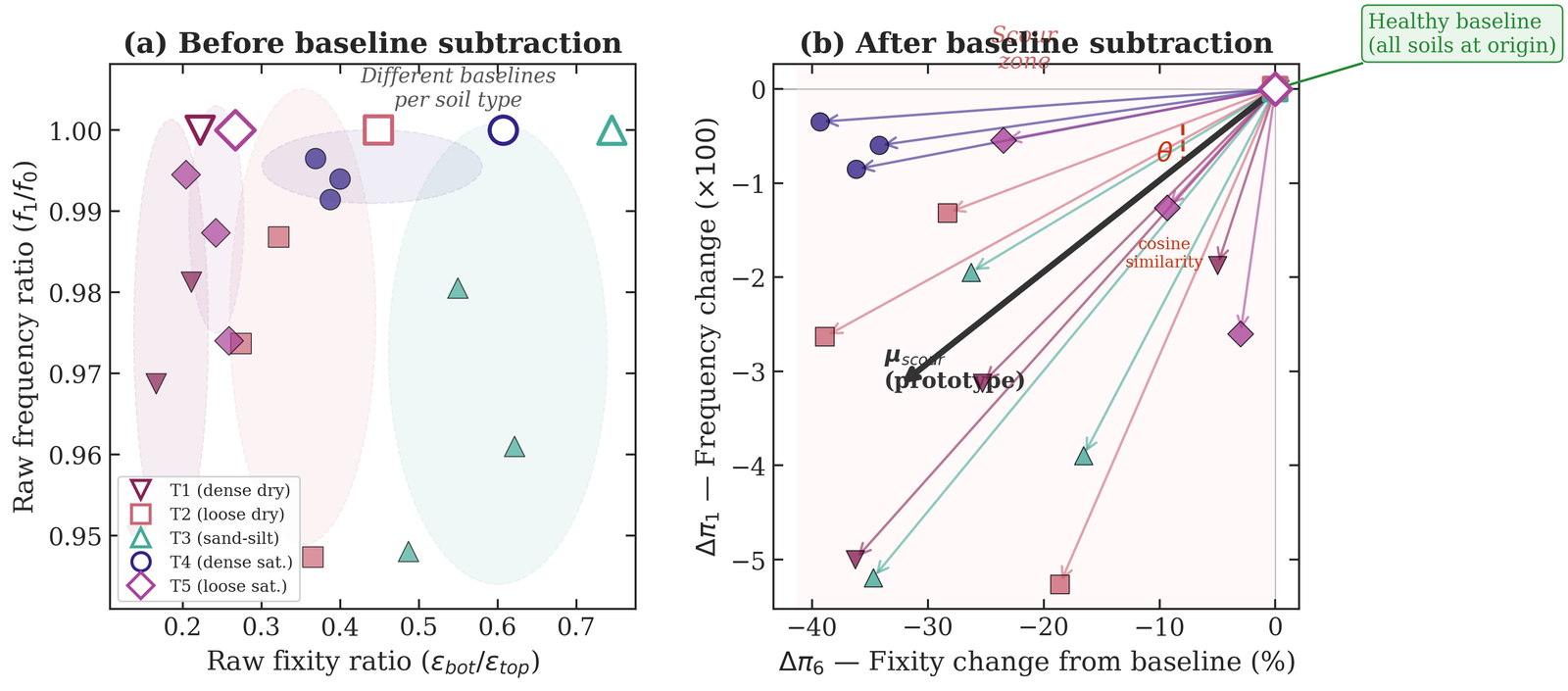
Figure 1: Baseline subtraction and damage vector construction. (a) Raw feature space with soil-dependent baselines. (b) After per-domain baseline subtraction, damage vectors radiate from the origin, and the scour prototype \(\boldsymbol{\mu}_{scour}\) defines the reference direction for cosine similarity classification.
A domain-specific baseline is computed independently for each dataset. For the centrifuge, the baseline is the mean feature vector across all no-scour (S/D = 0) windows from the same test series. For the field, the baseline is the mean over the first 12 months of monitoring, spanning a full annual cycle of tidal, thermal, and operational variability. The damage vector \(\Delta\boldsymbol{\pi}(t) = \boldsymbol{\pi}(t) - \boldsymbol{\pi}_0\) measures the deviation from the healthy state. Because all features are ratios normalized to the same baseline, this subtraction centres healthy observations at the origin in both domains, and cross-domain comparison requires only that the direction of scour-induced change be consistent, not that the absolute baseline values match.
In the centrifuge domain, the baseline-subtracted feature vector at each scour level is compared against the healthy state (the origin) through two mechanisms. For individual features, binary detection uses a simple sign test: if the normalized percentage change exceeds a threshold in the direction established by the centrifuge data (e.g., coherence increases, frequency decreases), the observation is flagged. For multivariate detection, the Mahalanobis distance from the healthy-state centroid measures the combined deviation across multiple features simultaneously, as described in Section 2.3.
The per-domain baseline strategy addresses a practical constraint. A joint baseline computed across both domains would require that the absolute feature values at the healthy state match between centrifuge and field. This requirement is violated in practice: boundary effects in the centrifuge strongbox, differences in soil fabric between pluviated laboratory sand and natural marine deposits, and installation-induced stress states in the field all shift the absolute feature values. Per-domain baselines relax this requirement to a weaker condition: that the direction of scour-induced change be consistent across domains, even if the absolute starting points differ. The backfill recovery stages in the centrifuge test programme (Section 3.1) provide an empirical test of this consistency, because backfill alters the structural state in a direction opposite to scour.
The field baseline was verified for stationarity by dividing the calibration period into quarterly segments and testing each for equivalence using a paired t-test (p > 0.05 indicates no significant difference). A Mann-Kendall trend test on \(f_1\) detected a statistically significant but practically negligible positive trend (\(\tau\) = +0.04, p \< 0.001), consistent with the large sample size (N = 4,513) rendering even trivial correlations formally significant; the trend magnitude corresponds to less than 0.1 mHz drift over the calibration year. A gold-standard comparison between the calmest month and the full year yielded a cosine similarity of 0.99. These checks provide confidence that the calibration period represents a stable structural state, although they cannot exclude the possibility that some degree of installation-induced or early-age scour is already incorporated in the baseline. If such pre-existing scour is present, the framework detects only changes beyond that initial state.
Detection framework
Two detection approaches are evaluated: single-feature thresholding and multivariate anomaly detection.
For single-feature detection, binary classification uses a threshold on the per-series normalized percentage change. Each candidate feature is tested independently: if the normalized value exceeds a threshold in the direction established by the centrifuge data (positive for coherence features, negative for frequency), the observation is flagged as scoured. A feature achieves binary separation if every scoured test across all soil conditions deviates from baseline in the same direction.
For multivariate detection, the Mahalanobis distance22 measures the joint deviation of multiple features from the healthy-state distribution:
where \(\Delta\boldsymbol{\phi}(t)\) is the vector of per-baseline-normalized feature values at time \(t\) and \(\boldsymbol{\Sigma}_0\) is the covariance matrix estimated from the calibration period. Unlike single-feature thresholding, the Mahalanobis distance accounts for the correlation structure between features and weights each feature direction by the inverse of its baseline variability. A feature that is noisy but directionally consistent with scour contributes less to the distance than a stable feature with the same signal magnitude. In the centrifuge, where only four to five healthy-state observations are available per soil, the covariance matrix cannot be reliably estimated for more than two to three features. In the field, the 12-month calibration period provides approximately 2,000 parked-condition windows, which is sufficient to estimate a four-dimensional covariance matrix.
For field deployment, an exponentially weighted moving average (EWMA) is applied to the Mahalanobis distance time series to reduce window-to-window variability. The smoothing span controls the trade-off between noise reduction and detection latency. An alarm is triggered when the EWMA-smoothed distance exceeds three standard deviations above the calibration-period mean, following standard statistical process control practice23. The projected signal-to-noise ratio (SNR) for each centrifuge scour level is computed by evaluating Eq. 1 at the centrifuge-measured feature shift and dividing by the EWMA-smoothed field standard deviation. An SNR above 2.0 indicates detectability at the 2\(\sigma\) level; above 3.0 indicates detectability at 3\(\sigma\).
Validation design
The absence of confirmed field scour events necessitates a multi-layered validation, because no single test can simultaneously verify sensitivity and specificity. For sensitivity, centrifuge data with known scour depths are used. Each of the 64 candidate features is evaluated for binary separation (healthy vs. any scour) across four soil conditions (T2 through T5, 16 tests). A feature achieves binary separation if every scoured test in every soil deviates from baseline in the same direction; the minimum percentage deviation across all scoured tests defines the separation margin. Leave-one-series-out (LOSO) cross-validation holds out each soil condition entirely and evaluates whether the detection threshold learned from the remaining soils correctly classifies the held-out soil, testing cross-soil generalisation. A permutation test (10,000 random label shuffles) verifies that the observed accuracy is not an artifact of the small sample size. Backfill recovery stages (T4-5 and T5-5) provide an independent check: if a feature responds to stiffness restoration after backfill, it responds to genuine structural change rather than to labelling artifacts.
For specificity, the 31-month field monitoring record serves as a prolonged negative control. Because no confirmed scour event occurred during the monitoring period, the field component tests only the false alarm rate, not detection of actual scour. The alarm rate is computed as the number of EWMA-smoothed observations exceeding the 3\(\sigma\) threshold. The projected detection capability is then quantified by computing the Mahalanobis-distance SNR that each centrifuge scour level would produce against the field noise floor, expressed as the ratio of the centrifuge signal magnitude to the EWMA-smoothed field standard deviation.
Experimental data
Prototype structure and site conditions
The reference structure for both the centrifuge model and the field monitoring is the UNISON U136 offshore wind turbine (rated capacity 4.2 MW, rotor diameter 136 m, hub height 96.3 m above mean sea level) installed at the Gunsan demonstration site in the Yellow Sea, South Korea. The turbine is supported by a tripod suction bucket foundation consisting of three steel buckets with diameter D = 8.0 m and skirt length L = 9.3 m, arranged in a triangular configuration at 20.0 m centre-to-centre spacing. The tower is a tapered S420ML steel tube (bottom diameter 4.2 m, top diameter 3.5 m) carrying a rotor-nacelle assembly of approximately 338 tonnes. The site water depth is 14 m at mean sea level.
The seabed at the Gunsan site comprises three distinct layers that govern both scour susceptibility and foundation behaviour. The upper layer (0 to 2.5 m below the seabed) is clean-to-silty sand, which is the primary scour-susceptible zone under wave-current action. Below this lies a low-plasticity silty clay layer extending from 2.5 to 8.3 m depth, with a coefficient of consolidation on the order of \(10^{-8}\) to \(10^{-7}\) m\(^2\)/s. The bucket skirt tips are embedded in a lower silty sand stratum from 8.3 to 10.8 m. This stratigraphy means that scour confined to the upper sand layer corresponds to a maximum normalised depth of S/D = 0.31 (2.5 m divided by 8.0 m bucket diameter). Scour beyond this depth would require erosion into the clay, which involves fundamentally different cohesive erosion mechanics, and falls outside the scope of the present centrifuge validation.
The structural dynamics of the prototype are governed by the interaction between the tower-foundation system and the surrounding soil. Bathymetric surveys conducted during installation documented local scour patterns around the buckets that informed the scour geometries adopted in the centrifuge programme. The scour-frequency sensitivity for this foundation type follows a power-law relationship \(\Delta f / f_0 = -0.12 (S/D)^{1.5}\), calibrated from centrifuge experiments on the same prototype5. This relationship predicts a 1.2% frequency reduction at S/D = 0.31 (the sand layer limit) and 3.5% at S/D = 0.58 (the maximum centrifuge scour depth), both within the range where environmental variability can mask the scour signal if only frequency is monitored. The tripod configuration introduces an additional complication relative to monopiles: under lateral loading, one bucket experiences uplift while the other two undergo compression, so that the net change in foundation stiffness depends on the direction of loading relative to the scour location and on the load redistribution capacity of the three-leg system6.
The choice of this particular prototype as the study subject is motivated by two considerations. First, the Gunsan turbine is one of a limited number of operating offshore wind turbines on tripod suction bucket foundations with both centrifuge test data and long-term field monitoring available for the same structure, enabling the cross-domain comparison that is central to this study. Second, the three-layer stratigraphy at the site provides a bounded validation envelope: the sand layer defines the scour conditions that the centrifuge can replicate, while the clay layer defines the boundary beyond which the present results do not apply. This bounded scope is stated as an explicit limitation rather than treated as a generalisation to all soil profiles.
Centrifuge test programme
The centrifuge experiments were conducted at the KAIST beam centrifuge24 (5.0 m effective radius, 2400 kg payload capacity) at a gravitational acceleration of 70g. The 1:70 scale model replicated the prototype tower geometry, tripod configuration, and rotor-nacelle assembly mass (1.08 kg model, equivalent to 370 tonnes at prototype scale, within 10% of the actual 338 tonne RNA). The model tower was fabricated from laser-welded ASTM-A240M stainless steel tubes (outer diameter 56.4 mm, wall thickness 0.5 mm), designed to match the prototype equivalent flexural rigidity EI within 2.3%. The model was housed in a rectangular aluminium strongbox (1400 mm by 650 mm by 700 mm) with Duxseal absorbing material applied to the walls to reduce wave reflections.
Instrumentation comprised 53 channels: 21 accelerometers (20 ADXL1003 MEMS devices at five tower elevations in biaxial configuration, plus one piezoelectric reference at the tower top), 12 strain gauges at three elevations (350, 750, and 1300 mm above the mudline in model scale), 10 Keyence laser displacement sensors (seven along the tower height plus three at bucket caps for differential settlement), five pore pressure transducers inside bucket A, and a dynamic load cell adjacent to the piezoelectric actuator. Dynamic excitation was applied via a Cedrat Technologies APA440MML amplified piezoelectric actuator mounted at the tower top, generating impulse, swept-sine (1 to 5 Hz model scale), and square-wave loading. Data were recorded at 5000 Hz for durations of 22 to 26 minutes per flight, producing 2.6 to 2.9 GB of raw data per test case.
Twenty test cases were performed across five series, each representing a distinct soil condition (Table 3). Each series included four progressive scour stages at normalised depths S/D ranging from 0 to 0.62, with series-specific values listed in Table 3. The T4 and T5 series included an additional backfill recovery stage in which coarser No. 5 sand (\(d_{50}\) = 1.99 mm) was placed around the buckets after maximum scour. Local scour was simulated by excavating sand around each bucket at 1g between centrifuge flights using a frustum-shaped concentric excavation tool, with the excavated soil mass verified for consistency. This procedure does not replicate progressive hydraulic erosion or the associated pore pressure transients. Initial frequency identification from broadband power spectral density showed an apparent T1 anomaly (frequency increasing with scour), attributed to densification artefacts during the 1g excavation procedure. The companion study’s optimised ringdown PSD extraction5 resolved this anomaly: all five series, including T1, exhibit monotonically decreasing frequencies with scour when the free-decay window is properly isolated (1.0 s Hann window, 50% overlap, parabolic peak interpolation within a 5 to 20 Hz search range), with inter-channel standard deviation of 0.005 to 0.012 Hz. The published natural frequencies from this optimised extraction are used throughout the present study. Full experimental details are reported in5,6.
Table 3: Centrifuge test matrix (20 test cases across five soil conditions). BF = backfill recovery stage using No. 5 sand (\(d_{50}\) = 1.99 mm). No. 7 sand has \(d_{50}\) = 0.21 mm; No. 8 sand-silt has \(d_{50}\) = 0.15 mm.
| Series | Soil condition | \(D_r\) (%) | Saturation | \(S/D\) values | Tests |
|---|---|---|---|---|---|
| T1 | Dense sand (No. 7) | 83 | Dry | 0, 0.20, 0.33, 0.48 | 4 |
| T2 | Loose sand (No. 7) | 58 | Dry | 0, 0.30, 0.43, 0.62 | 4 |
| T3 | Sand-silt (No. 8) | 57 | Dry | 0, 0.29, 0.49, 0.56 | 4 |
| T4 | Dense sand (No. 7) | 70 | Saturated | 0, 0.19, 0.39, 0.58 + BF | 5 |
| T5 | Loose sand (No. 7) | 61 | Saturated | 0, 0.19, 0.39, 0.58 + BF | 5 |
Field monitoring campaign
The same prototype structure was monitored continuously from May 2023 to December 2025 (31 months) across 47 data-acquisition campaigns. The structural monitoring system comprised 11 channels at three tower elevations: three accelerometers at 1500 Hz and eight strain gauges at 500 Hz. The accelerometers are located at the tower base (Node 100, 23.6 m above mean sea level), while strain gauges span all three elevations: tower base (Node 100, 23.6 m), tower mid (Node 108, 44.3 m), and hub height (Node 127, 96.3 m). Each elevation carries bidirectional bending channels (east-west and north-south), plus a torsion channel at the tower top. The tower-mid east-west bending channel (WTOW-Tmd-EWBnd), present in the data acquisition system but omitted from the companion study’s processing pipeline25, was recovered in this study from the raw binary sensor files, providing complete bidirectional strain measurements at all three elevations.
Modal parameters were extracted using covariance-driven stochastic subspace identification (SSI-COV)26 with automated pole clustering25. The SSI-COV implementation used 600-second analysis windows, decimation from native sampling rates to 50 Hz, Hankel matrix dimensions of 80 block rows and columns, and model order sweeps from 20 to 100 in steps of 2. A modal assurance criterion (MAC) threshold of 0.85 against a finite-element reference model served as the quality gate, retaining 6,878 of 22,616 total windows (30.4%), corresponding to approximately 7.3 modal estimates per day. The identified first natural frequency was 243.3 mHz with a raw standard deviation of 3.72 mHz (1.53% coefficient of variation). The companion study25 applied a physics-informed normalization framework to this frequency data, achieving a post-normalization standard deviation of 1.11 mHz and zero structural alarms over the monitoring period. This zero-alarm result provides the basis for treating the entire field record as a healthy-state reference in the present study.
Raw strain time-series were separately extracted from the original binary sensor files across all 47 campaign folders, producing 23,252 ten-minute windows. The extraction was necessary because the companion study computed curvature at the tower base only and did not produce per-elevation strain amplitudes, fixity ratios, or cross-sensor spectral features required for the present analysis. Each window was detrended and bandpass-filtered between 0.05 and 2.0 Hz using a fourth-order Butterworth filter implemented in second-order sections for numerical stability. Strain root-mean-square amplitudes were computed independently at each elevation, and the fixity ratio was formed as the bottom-to-top amplitude ratio. Environmental and operational data (tidal level, temperature, rotor speed, and current velocity reconstructed from tidal harmonic analysis of nine astronomical constituents at three KHOA oceanographic stations) were synchronized with the structural measurements.
The turbine operates in distinct regimes that affect the strain distribution differently. When the rotor is turning (speed above 2 rpm), centrifugal forces, aerodynamic loading, and blade-passing harmonics contribute to the broadband strain, and the fixity ratio correlates strongly with rotor speed (Pearson \(r\) = -0.76). When the turbine is parked (speed below 2 rpm), the structure responds primarily to wave and wind forcing, and the fixity ratio becomes nearly independent of all measured environmental variables (|\(r\)| \< 0.08 for tidal level, temperature, and current speed). This regime dependence motivated the parked-only filtering strategy adopted in the field validation, which eliminates the dominant confounder at the cost of reducing the merged dataset to approximately 45% (3,355 of 7,492 windows with matching environmental data). The merging step itself reduces the 23,252 raw strain windows to 7,492 because environmental and operational data were not available for all campaigns.
Cross-domain sensor correspondence and processing harmonization
Fig. 2 illustrates the sensor positions in both domains mapped onto a normalised tower elevation diagram. The centrifuge model has strain gauges at three elevations and accelerometers at five, while the field system has strain gauges at three elevations and accelerometers at the tower base. The bottom strain gauge positions are closely matched in normalised height (\(z/H\) = 0.24 in both domains), which is the elevation most sensitive to changes in the effective fixity point.
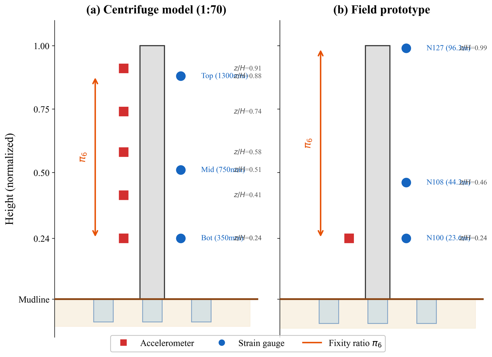
Figure 2: Cross-domain sensor layout showing centrifuge model (left) and field prototype (right). Sensor positions are mapped to normalised tower height \(z/H\). The strain-acceleration coherence \(\phi_4\) is computed between the mid-elevation strain gauge and the accelerometer in each domain.
The strain fixity ratio requires strain measurements at two tower elevations in each domain. In the centrifuge model, strain gauges are located at 350 mm and 1300 mm above the mudline (normalised heights \(z/H\) = 0.24 and 0.88, where \(H\) = 1478 mm is the total model height). In the field, the corresponding channels are at Node 100 (23.6 m, \(z/H\) = 0.24) and Node 127 (96.3 m, \(z/H\) = 0.99). The bottom sensor positions are well-matched in normalised height, while the top sensor is closer to the hub in the field than in the centrifuge. This mismatch means the absolute fixity ratio differs between domains: centrifuge baseline values range from 0.22 to 0.74 across soils, while the field baseline under parked conditions is 7.0. The per-domain baseline subtraction described in Section 2.2 removes this offset, and the validity of this approach is supported by centrifuge data showing that fixity ratios computed from different elevation pairs (bottom-to-mid and bottom-to-top) produce consistent percentage decreases under scour.
Signal processing differs between domains in three respects. First, the excitation source is deterministic in the centrifuge (piezoelectric actuator producing impulse and swept-sine loading) and stochastic in the field (ambient wind and wave forcing supplemented by rotor harmonics); broadband strain ratios are less affected than absolute amplitudes because both numerator and denominator scale with the same excitation input. Second, the sampling rates differ (5000 Hz centrifuge vs. 500 Hz field strain), affecting frequency resolution of spectral features but not the time-domain amplitude ratios used for fixity computation. Third, natural frequency is identified through Welch periodogram peak-picking in the centrifuge and SSI-COV in the field; the frequency ratio \(\pi_1\) is insensitive to the identification method because the ratio cancels any systematic bias between methods (Supplementary Material S5). The three-tier classification in Table 2 reflects these processing differences: features robust to all three are classified as rigorously invariant, while those sensitive to excitation type are classified as conditionally invariant.
The hydrodynamic similitude gap between the two domains warrants explicit discussion. The centrifuge tests model the soil-structure system under controlled mechanical excitation without wave or current loading, whereas the field structure is subjected to continuous hydrodynamic forcing that contributes both quasi-static and dynamic loads. Because the non-dimensional features used in this study are baseline-normalised ratios (current value divided by healthy-state value from the same domain), hydrodynamic effects that are present in both the numerator and denominator of the field ratios cancel to first order. The residual hydrodynamic contribution appears as additional variance in the field features, which is quantified through the calibration-period statistics and managed through the EWMA smoothing and parked-condition filtering described in Section 3.3. The centrifuge does not need to replicate the wave environment for the cross-domain comparison to hold; it needs only to produce the correct relationship between scour depth and the structural feature response, which the dimensional analysis framework ensures through the scale-invariance proofs presented in Section 2.1.
A summary of the cross-domain mapping for each retained feature illustrates the practical correspondence. For the frequency ratio \(\pi_1\), the centrifuge provides f\(_1\) via Welch periodogram at 5000 Hz and the field provides f\(_1\) via SSI-COV at 50 Hz (after decimation from 1500 Hz); both estimate the same physical quantity (the first bending mode frequency) with sub-percent precision. For the strain fixity ratio \(\pi_6\), the centrifuge uses strain gauges at \(z/H\) = 0.24 and 0.88 under deterministic excitation, while the field uses gauges at \(z/H\) = 0.24 and 0.99 under ambient excitation; the per-domain baseline subtraction removes the absolute offset arising from the sensor height mismatch, and the parked-condition filter removes the excitation-dependent variance. For the conditionally invariant features (coherence \(\pi_7\) and spectral entropy \(\pi_{11}\)), the cross-domain comparison is less secure because coherence is sensitive to the bandwidth and stationarity of the excitation; these features are retained for centrifuge-internal analysis and diagnostic purposes but are not used for cross-domain binary detection, which relies solely on the rigorously invariant \(\pi_6\) (fixity) and \(\pi_1\) (frequency).
Results and Discussion
Comprehensive feature evaluation
Sixty-four non-dimensional features were computed from the x-direction strain and acceleration channels for each of the 16 centrifuge test cases (T2 through T5, four scour stages each). Faulty channels were excluded: for T4, the y-direction bottom strain gauges (str_bot_y_1 and str_bot_y_2) showed anomalous values at baseline (13.5 and 0.0 respectively, compared to 0.88 for the x-direction channels) and were removed from all analyses. Each feature was normalised by its per-series healthy-state baseline, and binary separation was assessed by checking whether every scoured test across all four soils deviated from baseline in the same direction.
Of the 64 features tested, only two achieve binary separation across all four soils (Table 4). Both are coherence-based: the mid-acceleration strain coherence at \(f_1\) (\(\phi_4\) computed between the mid-elevation strain gauge and the tower-top accelerometer) and its band-averaged variant. The conventional strain fixity ratio (\(\phi_3\), bottom-to-top amplitude) fails in two of four soils (T3 and T5 show mixed sign changes with scour). All spectral entropy features, PSD ratios, and transfer function magnitudes also fail to achieve consistent 4/4 separation.
Table 4: Binary separation results for selected features (16 tests, 4 soils). A feature achieves separation if every scoured test in every soil deviates from baseline in the same direction. Min. margin is the smallest absolute percentage deviation of any scoured test from zero. The frequency ratio (\(\phi_1\), published values from5) achieves 5/5 separation across all five soils including T1 (not shown here because T1 strain data was processed with a different method).
| Feature | Category | 4/4 separation | Min. margin | Direction |
|---|---|---|---|---|
| Coherence mid-accel (band) | \(\phi_4\) variant | Yes | 8.8% | Increases |
| Coherence mid-accel (at \(f_1\)) | \(\phi_4\) | Yes | 7.4% | Increases |
| Coherence mid-top (at \(f_1\)) | strain-strain | 3/4 | 5.6% | Increases |
| Coherence bot-top (band) | strain-strain | 3/4 | 1.1% | Increases |
| Fixity ratio bot/top | \(\phi_3\) | 2/4 | – | Mixed |
| Fixity ratio bot/mid | \(\phi_3\) variant | 2/4 | – | Mixed |
| Spectral entropy ratio | \(\phi_5\) | 0/4 | – | Mixed |
| Strain amplitude ratio | \(\phi_2\) | 0/4 | – | Mixed |
Fig. 3 illustrates the contrast between the two feature types. The fixity ratio (panel a) shows mixed-sign changes with no consistent direction across soils, while the mid-acceleration coherence (panel b) increases in every soil after every scour increment, with a minimum margin of 8.8%.
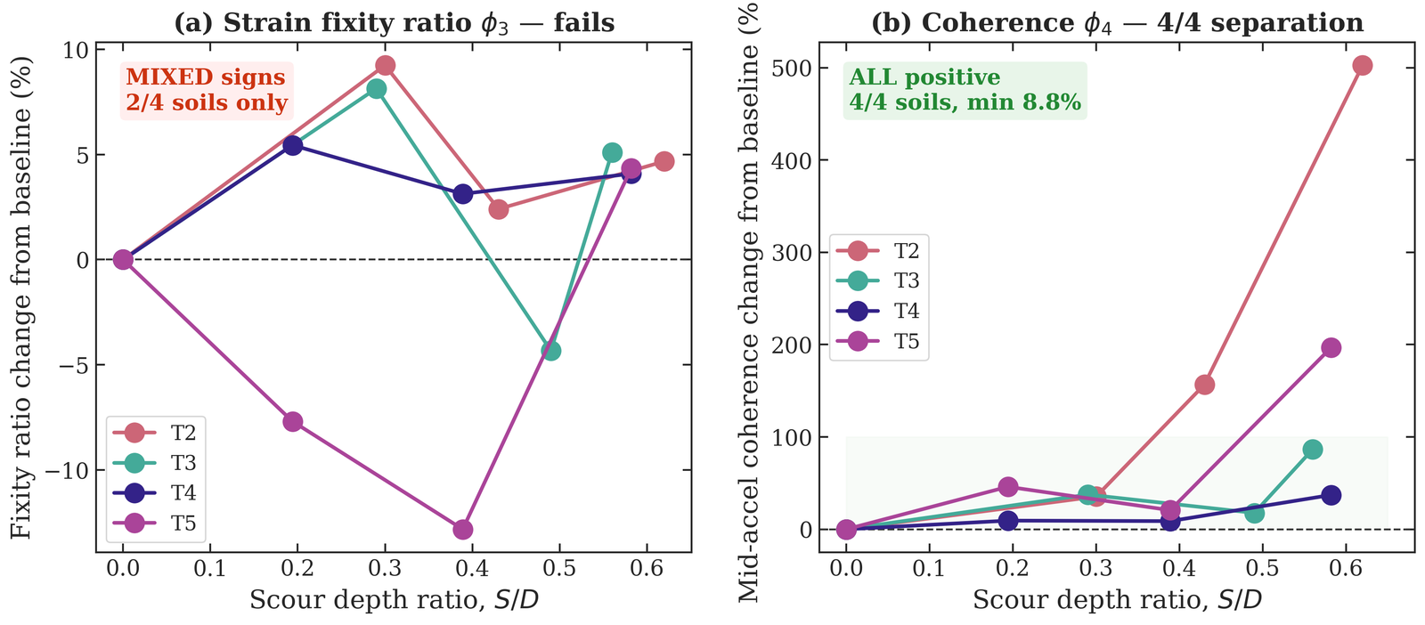
Figure 3: Binary separation comparison. (a) Strain fixity ratio (\(\phi_3\), x-direction) shows inconsistent sign across soils and fails binary detection. (b) Mid-acceleration coherence (\(\phi_4\), band-averaged at \(f_1\)) increases under scour in all four soils with a minimum margin of 8.8%.
The mid-acceleration coherence succeeds because scour softens the foundation and concentrates the structural response at the first bending mode. At the mid-elevation strain gauge, the fraction of broadband strain energy attributable to \(f_1\) increases as higher modes become less significant relative to the fundamental. The coherence between mid-strain and acceleration at \(f_1\) directly measures this concentration. The percentage changes are large: T2 increases by 35% at minimum and T5 by 21%, with T3 and T4 showing smaller but consistently positive changes (17.7% and 8.8% respectively).
The strain fixity ratio (\(\phi_3\)), by contrast, fails binary separation because its sign is inconsistent across soils when computed from correctly isolated x-direction channels. In T3 (sand-silt), the fixity ratio increases at S/D = 0.29 (+8.1%) before decreasing at S/D = 0.49 (-4.3%), producing a mixed-sign pattern that no single threshold can classify. T5 (loose saturated) shows a similar non-monotonic pattern driven by the bending-to-tilting regime transition documented in6. The original analysis, which reported monotonic fixity decreases, was based on time-domain averaging of orthogonal (x and y direction) strain channels, which introduced an artificial amplitude-dependent distortion. When the channels are correctly separated by bending direction, the fixity ratio produces only 2-13% total variation with inconsistent sign across soils.
A permutation test (10,000 random label shuffles) confirms that the 100% binary accuracy of the mid-acceleration coherence is statistically significant (p = 0.0003). Leave-one-series-out cross-validation yields 100% accuracy for all four held-out soils, with detection margins ranging from 8.8% (T4) to 35.4% (T2). The published frequency ratio (\(\phi_1\)) independently achieves 100% LOSO accuracy across all five soils (including T1), with margins ranging from 0.35% (T4-S1) to 5.26% (T2-S3). Per-test feature values and LOSO results are provided in Supplementary Material S2 and S3.
Field environmental sensitivity
Field strain and coherence features were computed from 23,252 ten-minute windows across 47 monitoring campaigns. Of these, 7,492 have matching environmental data and 3,355 correspond to parked conditions (rotor speed below 2 rpm). Table 5 reports the absolute Pearson correlation between each feature and four environmental variables during the calibration year under parked conditions.
Table 5: Environmental correlation of field features under parked conditions (calibration period, n = 1,989 windows). The mid-acceleration coherence has the lowest maximum correlation with any environmental variable (|\(r\)| = 0.092), followed by frequency (0.117).
| Feature | Rotor speed | Tidal level | Temperature | Current speed | Max |
|---|---|---|---|---|---|
| Frequency (\(\phi_1\)) | 0.058 | 0.027 | 0.117 | 0.077 | 0.117 |
| Fixity ratio (\(\phi_3\)) | 0.173 | 0.044 | 0.127 | 0.047 | 0.173 |
| Coherence mid-accel (\(\phi_4\)) | 0.073 | 0.029 | 0.034 | 0.092 | 0.092 |
| Coherence bot-top | 0.109 | 0.078 | 0.005 | 0.188 | 0.188 |
The mid-acceleration coherence is the least environmentally sensitive strain-based feature (max |\(r\)| = 0.092). The fixity ratio, despite producing zero individual-feature alarms in the field, has the highest rotor-speed correlation (0.173) among the features considered. The frequency feature has low environmental sensitivity (max |\(r\)| = 0.117) consistent with the companion study’s normalisation results25.
Multivariate field detection
Individual features face a fundamental trade-off: the mid-acceleration coherence has strong centrifuge sensitivity (8.8% minimum margin) but drifts in the field (196 alarms at EWMA-384 with fixed baseline), while the frequency ratio has excellent field stability (zero alarms, \(\sigma\) = 0.2% at EWMA-384) but weak centrifuge sensitivity in dense saturated sand (0.35% at S/D = 0.19). A multivariate Mahalanobis anomaly detector resolves this trade-off by combining both features through their joint calibration-period covariance.
The field calibration period (first 12 months, 1,989 parked windows) provides the healthy-state mean \(\boldsymbol{\mu}_0\) and covariance \(\boldsymbol{\Sigma}_0\) in the two-dimensional feature space (frequency change, coherence change). The Mahalanobis distance is computed for each subsequent window, EWMA-smoothed at span 384, and thresholded at 3\(\sigma\) above the calibration-period mean. Table 6 reports the projected signal-to-noise ratio for each centrifuge scour level, computed by evaluating the Mahalanobis distance at the centrifuge-measured feature shift and dividing by the EWMA-smoothed field standard deviation.
Table 6: Projected signal-to-noise ratio for the multivariate detector (frequency + mid-accel coherence, Mahalanobis distance, EWMA-384). Zero alarms over the 31-month monitoring period. All scour levels exceed SNR = 2.0 (2\(\sigma\) detection). All moderate-to-severe scour (S2, S3) exceeds SNR = 3.0 (3\(\sigma\) detection). The weakest case is T4-S1 (dense saturated, S/D = 0.19) at SNR = 2.2.
| Soil | S/D (S1) | SNR (S1) | S/D (S2) | SNR (S2) | S/D (S3) | SNR (S3) |
|---|---|---|---|---|---|---|
| T2 (loose dry) | 0.30 | 8.2 | 0.50 | 18.5 | 0.60 | 43.9 |
| T3 (sand-silt) | 0.20 | 12.0 | 0.30 | 23.5 | 0.50 | 31.8 |
| T4 (dense sat.) | 0.19 | 2.2 | 0.39 | 3.7 | 0.58 | 5.6 |
| T5 (loose sat.) | 0.19 | 4.3 | 0.39 | 7.7 | 0.58 | 19.7 |
Fig. 4 presents the projected SNR for each soil and scour level.
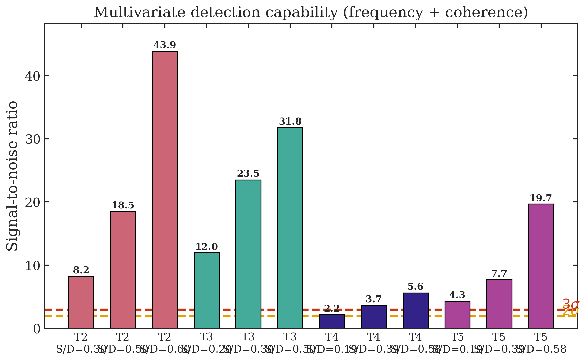
Figure 4: Multivariate detection capability: projected signal-to-noise ratio for each centrifuge scour level using the frequency + mid-accel coherence Mahalanobis detector with EWMA-384 smoothing. Dashed lines indicate the 2\(\sigma\) and 3\(\sigma\) detection thresholds. Zero alarms over 31 months of field monitoring.
Every scour level in every soil condition is detectable at the 2\(\sigma\) level or better. All moderate and severe scour levels exceed the 3\(\sigma\) threshold. The weakest detection point is T4-S1 (dense saturated sand at S/D = 0.19) at SNR = 2.2, corresponding to a scour depth of approximately 1.6 m around an 8.0 m diameter bucket. The multivariate detector succeeds where individual features fail because the Mahalanobis distance weights each feature by the inverse of its calibration-period variance: coherence adds information where frequency is weak (T4, T5), while stable frequency prevents noisy coherence from triggering false alarms.
The non-stationarity of the mid-acceleration coherence, which produces 196 alarms when used as a single-feature detector, does not propagate to the multivariate alarm because environmental coherence drift is not accompanied by a systematic frequency shift. The covariance structure of the healthy-state distribution distinguishes scour-consistent joint deviations from environmentally driven single-feature drift.
Fig. 5 shows the field time series for both features over the 31-month monitoring period.
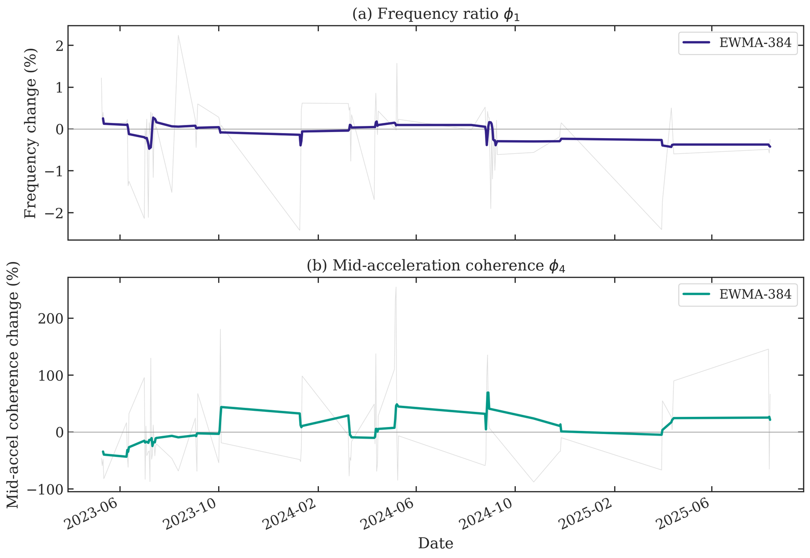
Figure 5: Field time series of (a) frequency ratio and (b) mid-acceleration coherence over 31 months of parked-condition monitoring. Grey: daily-median raw values. Coloured lines: EWMA-384 smoothed values. Both features remain within the calibration-period variability throughout the monitoring period.
The EWMA step response at span 384 follows \(y(t) = 1 - (1-\alpha)^t\) with \(\alpha = 0.0052\), reaching 50% of a step change after approximately 38 days and 95% after 164 days. This latency is acceptable for scour monitoring of suction bucket foundations, where erosion is a long-term morphological process driven by seasonal storm cycles.
Comparison with existing approaches
Only three prior studies have attempted cross-domain transfer for scour detection, and none addresses multi-footing foundations.11 used a finite-element digital twin for monopile scour detection, achieving detection of 0.05D scour within two weeks.15 applied Naive Bayes classification to numerically simulated acceleration features, achieving 94% on simulated data without cross-domain validation.17 attempted centrifuge-to-field frequency transfer for bridge scour but found that field measurement uncertainty exceeded the scour signal.
Table 7: Comparison of cross-domain scour detection approaches.
| Criterion | 11 | 15 | 17 | This study |
|---|---|---|---|---|
| Source domain | FEM digital twin | FEM simulation | Centrifuge | Centrifuge |
| Target domain | Field (monopile) | Simulated only | Field (bridge) | Field (TSB, 31 months) |
| Domain bridge | Model calibration | None (same domain) | Frequency scaling | Buckingham Pi |
| Features | Frequency only | Acceleration PCA | Frequency only | Frequency + coherence (multivariate) |
| EOV handling | Tree-based ML | None | None | Parked filter + Mahalanobis covariance |
| Foundation type | Monopile | Monopile | Bridge pile | Tripod suction bucket |
| Detection | 0.05D in 2 weeks | 94% (simulated) | Failed | All S/D \(\geq\) 0.19 at 2\(\sigma\) |
The multivariate approach addresses the limitation that prevented transfer in17: by combining frequency with strain-acceleration coherence, the detector achieves sufficient SNR even when the frequency signal alone falls below the field noise floor. Population-based SHM27,28 addresses transfer between structures within a fleet; the present study addresses transfer between scales using Buckingham Pi analysis as the domain bridge.
Limitations
Several limitations require explicit statement. First, no confirmed scour event occurred during the 31-month monitoring period. The field validation tests specificity (zero alarms) but not sensitivity. All projected SNR values combine centrifuge-calibrated signal magnitudes with the field noise floor and have not been verified against actual field scour. Coordinated vibration and bathymetric monitoring campaigns remain the definitive validation path. Second, the cross-soil transfer spans four sand and sand-silt conditions but does not extend to cohesive soils. Scour into the marine clay layer (below 2.5 m at the Gunsan site) involves different erosion mechanics, and the coherence response to clay erosion has not been tested. Third, the absolute coherence values differ by an order of magnitude between centrifuge (0.01 to 0.96) and field (0.26 mean), so cross-domain comparison operates exclusively through percentage change from per-domain baselines. Whether the same percentage coherence change corresponds to the same physical scour depth in both domains cannot be confirmed without an actual field scour event. Fourth, the strain fixity ratio, which was the original candidate feature for this study, fails binary separation when the strain channels are correctly separated by bending direction. The previously reported fixity-based results were based on time-domain averaging of orthogonal strain components, which introduced an artificial distortion. This negative finding is reported to prevent its propagation in the literature.
Conclusions
A systematic evaluation of 64 non-dimensional features derived from Buckingham Pi analysis reveals that the strain-acceleration coherence at the first natural frequency is the only strain-based feature that consistently separates healthy from scoured states across four soil conditions in centrifuge tests on a 1:70 scale model of a 4.2 MW tripod suction bucket foundation. The strain fixity ratio, which has been assumed to be an effective scour indicator, fails binary separation when the strain channels are correctly separated by bending direction. This negative result has not been reported previously and redirects the search toward cross-spectral features rather than amplitude ratios.
Combined with the published natural frequency ratio, the mid-acceleration coherence forms a two-feature multivariate Mahalanobis detector that achieves zero alarms over 31 months of field monitoring while maintaining a projected signal-to-noise ratio above 2.0 for the mildest centrifuge scour level (S/D = 0.19) in every soil condition tested. The multivariate approach resolves the individual-feature trade-off: frequency provides field stability but weak sensitivity in dense saturated sand, while coherence provides centrifuge sensitivity but non-stationary field behaviour. The joint covariance structure distinguishes scour-consistent multi-feature deviations from environmentally driven single-feature drift.
Among published cross-domain scour detection studies, this is the first to achieve experimentally validated transfer from a centrifuge model to a field-deployed prototype for a multi-footing offshore foundation. The Buckingham Pi framework provides the domain bridge: by expressing all features as deviations from per-domain baselines of dimensionless quantities, the scaling factor cancels and centrifuge-calibrated damage signatures become directly applicable to field deployment without statistical domain adaptation.
Statements and declarations
Declaration of conflicting interests
The author(s) declared no potential conflicts of interest with respect to the research, authorship, and/or publication of this article.
Funding
This research was supported by the Korea Electric Power Corporation (Grant number: R23XO05-01) and the National Research Foundation of Korea (NRF) grant funded by the Korea government (MSIT) (RS-2022-NR070302).
Data availability
The centrifuge data supporting the findings of this study are available from the corresponding author upon reasonable request. Field monitoring data are subject to restrictions under the KEPCO collaborative agreement and are not publicly available.
References
Supplementary Material
S1. Buckingham Pi derivation
S1.1 Governing dimensional quantities
The dynamic response of the tripod suction bucket system under progressive scour is governed by twelve dimensional quantities:
| # | Symbol | Quantity | Dimensions |
|---|---|---|---|
| 1 | \(f_n\) | Natural frequency | \([\text{T}^{-1}]\) |
| 2 | \(a_\text{rms}\) | RMS acceleration | \([\text{LT}^{-2}]\) |
| 3 | \(\varepsilon\) | Strain | \([-]\) (dimensionless) |
| 4 | \(D\) | Bucket diameter | \([\text{L}]\) |
| 5 | \(L_\text{sk}\) | Skirt length | \([\text{L}]\) |
| 6 | \(H\) | Tower height | \([\text{L}]\) |
| 7 | \(S\) | Scour depth | \([\text{L}]\) |
| 8 | \(m_\text{RNA}\) | RNA mass | \([\text{M}]\) |
| 9 | \(\rho_s\) | Soil density | \([\text{ML}^{-3}]\) |
| 10 | \(G_0\) | Small-strain shear modulus | \([\text{ML}^{-1}\text{T}^{-2}]\) |
| 11 | \(EI\) | Tower flexural rigidity | \([\text{ML}^{3}\text{T}^{-2}]\) |
| 12 | \(\gamma'\) | Effective unit weight | \([\text{ML}^{-2}\text{T}^{-2}]\) |
With \(n = 12\) quantities (excluding \(\varepsilon\), which is inherently dimensionless) and \(k = 3\) fundamental dimensions \([M, L, T]\), the Buckingham Pi theorem yields \(m = 9\) independent dimensionless groups.
S1.2 Repeating variables and dimensional independence
The repeating variables \(\{D, \rho_s, G_0\}\) are selected as independent system properties (not response quantities). Their dimensional exponent matrix:
has determinant 2 \(\neq\) 0, confirming dimensional independence.
S1.3 Derivation of fundamental Pi groups
Each group is formed by combining a non-repeating variable with powers of the repeating variables such that all dimensions cancel.
\(\Pi_1\) from \(f_n\): Requiring \([T^{-1}][L]^a[ML^{-3}]^b[ML^{-1}T^{-2}]^c = [M^0L^0T^0]\) yields \(a=1\), \(b=1/2\), \(c=-1/2\):
\(\Pi_2\) from \(a_\text{rms}\): Similarly:
Geometric and mass groups:
S1.4 Scale-invariance proofs for monitoring features
Under \(N\)-g centrifuge scaling (\(N=70\)): frequency scales as \(N\), strain scales as 1:1, and \(G_0 \approx 1\) (at identical effective stress). The five monitoring features inherit their invariance from the fundamental groups:
\(\pi_1 = f_1/f_0\) (frequency ratio): \(\pi_{1,m} = (Nf_{1,p})/(Nf_{0,p}) = f_{1,p}/f_{0,p} = \pi_{1,p}\) \(\checkmark\) (rigorous)
\(\pi_3 = \varepsilon_\text{rms}/\varepsilon_0\) (strain ratio): \(\pi_{3,m} = \varepsilon_p/\varepsilon_{0,p} = \pi_{3,p}\) \(\checkmark\) (rigorous)
\(\pi_6 = \varepsilon_\text{bot}/\varepsilon_\text{top}\) (fixity ratio): Ratio of two dimensionless quantities; trivially invariant \(\checkmark\) (rigorous)
\(\pi_7 = \text{Coh}(a, \varepsilon)\) at \(f_1\) (coherence): Ratio of spectral densities is amplitude-invariant, but sensitive to excitation bandwidth \(\checkmark^*\) (conditional)
\(\pi_{11} = H_\text{spec}/H_0\) (spectral entropy ratio): Normalised PSD makes entropy insensitive to absolute amplitude; requires matched \(\Delta f/f_1\) \(\checkmark^*\) (conditional)
S2. Per-test feature values
Table 8: Per-test feature values for T1-T5. \(f_1\) is model-scale frequency from optimised ringdown PSD5. Coh\(_{ma}\) is the mid-acceleration strain coherence at \(f_1\) (band-averaged, x-direction). \(\Delta\phi_1\) and \(\Delta\phi_4\) are percentage deviations from the per-series S0 baseline. T1 coherence is not available because T1 strain data was processed with a different method.
| Test | Series | \(S/D\) | Level | \(f_1\) (Hz) | Coh\(_{ma}\) | \(\Delta\phi_1\) (%) | \(\Delta\phi_4\) (%) |
|---|---|---|---|---|---|---|---|
| T1-1 | T1 | 0.00 | S0 | 11.20 | – | 0.00 | – |
| T1-2 | T1 | 0.20 | S1 | 10.99 | – | -1.87 | – |
| T1-3 | T1 | 0.33 | S2 | 10.85 | – | -3.12 | – |
| T1-4 | T1 | 0.48 | S3 | 10.64 | – | -5.00 | – |
| T2-1 | T2 | 0.00 | S0 | 10.64 | 0.0026 | 0.00 | 0.0 |
| T2-2 | T2 | 0.30 | S2 | 10.50 | 0.0036 | -1.32 | +35.4 |
| T2-3 | T2 | 0.43 | S2 | 10.36 | 0.0068 | -2.63 | +156.7 |
| T2-4 | T2 | 0.62 | S3 | 10.08 | 0.0159 | -5.26 | +502.6 |
| T3-1 | T3 | 0.00 | S0 | 10.78 | 0.0093 | 0.00 | 0.0 |
| T3-2 | T3 | 0.29 | S2 | 10.57 | 0.0129 | -1.95 | +37.6 |
| T3-3 | T3 | 0.49 | S3 | 10.36 | 0.0110 | -3.90 | +17.7 |
| T3-4 | T3 | 0.56 | S3 | 10.22 | 0.0174 | -5.19 | +86.5 |
| T4-1 | T4 | 0.00 | S0 | 10.92 | 0.5367 | 0.00 | 0.0 |
| T4-2 | T4 | 0.19 | S1 | 10.88 | 0.5869 | -0.35 | +9.4 |
| T4-3 | T4 | 0.39 | S2 | 10.85 | 0.5841 | -0.60 | +8.8 |
| T4-4 | T4 | 0.58 | S3 | 10.83 | 0.7360 | -0.85 | +37.1 |
| T5-1 | T5 | 0.00 | S0 | 10.78 | 0.0193 | 0.00 | 0.0 |
| T5-2 | T5 | 0.19 | S1 | 10.73 | 0.0283 | -0.55 | +46.0 |
| T5-3 | T5 | 0.39 | S2 | 10.65 | 0.0233 | -1.26 | +20.6 |
| T5-4 | T5 | 0.58 | S3 | 10.50 | 0.0574 | -2.60 | +196.7 |
S3. Leave-one-series-out cross-validation detail
Binary LOSO for the mid-acceleration coherence uses a positive-change threshold: observations with \(\Delta\phi_4 > 0.5\%\) are classified as scoured. The threshold is physics-derived (scour increases coherence), not data-fitted. LOSO for the frequency ratio uses a negative-change threshold: \(\Delta\phi_1 < -0.1\%\).
Table 9: LOSO binary classification results for coherence (\(\phi_4\)) and frequency (\(\phi_1\)). Min. coh. margin is the smallest coherence percentage change from baseline for any scoured test in the held-out series.
| Held-out series | \(n\) tests | Coh. TP | Coh. TN | Coh. accuracy | Freq. accuracy | Min. coh. margin |
|---|---|---|---|---|---|---|
| T2 (loose dry) | 4 | 3 | 1 | 100% | 100% | 35.4% |
| T3 (sand-silt) | 4 | 3 | 1 | 100% | 100% | 17.7% |
| T4 (dense sat.) | 4 | 3 | 1 | 100% | 100% | 8.8% |
| T5 (loose sat.) | 4 | 3 | 1 | 100% | 100% | 20.6% |
The permutation test (10,000 random label shuffles) yields p = 0.0003 for coherence binary accuracy, confirming that the separation is not an artifact of the sample size.
S4. EWMA detection analysis
S4.1 EWMA step response
The exponentially weighted moving average with span \(s\) has smoothing parameter \(\alpha = 2/(s+1)\). The response to a unit step change at \(t=0\) is:
For the selected span \(s=384\) (\(\alpha = 0.0052\)):
- 50% response: 133 windows \(\approx\) 38 days
- 95% response: 575 windows \(\approx\) 164 days
where the conversion uses the observed rate of 3.5 parked windows per day.
S4.2 False alarm rate vs. smoothing span
The number of 3\(\sigma\) threshold exceedances during the 31-month monitoring period as a function of EWMA span:
Table 10: 3\(\sigma\) alarm count as a function of EWMA smoothing span during the monitoring period. The minimum span for zero alarms is 96 windows (approximately 27 days).
| EWMA span | Approx. days | \(\sigma\) (%) | 3\(\sigma\) alarms |
|---|---|---|---|
| 12 | 3 | 29.5 | 24 |
| 24 | 7 | 25.3 | 19 |
| 36 | 10 | 22.7 | 12 |
| 48 | 14 | 20.7 | 8 |
| 60 | 17 | 19.2 | 5 |
| 72 | 21 | 17.9 | 3 |
| 96 | 27 | 16.1 | 0 |
| 192 | 55 | 11.9 | 0 |
| 384 | 110 | 8.4 | 0 |
The selected span of 384 is conservative relative to the zero-alarm boundary at 96, providing additional margin against non-stationary noise sources. At span 384, the minimum detectable scour at 3\(\sigma\) is a fixity change of \(3 \times 8.4 = 25.1\%\), corresponding approximately to S2-equivalent scour. At 2\(\sigma\), the minimum detectable change is \(16.7\%\), which falls between the minimum S1 signal (-5%) and the mean S1 signal (-23%).
S5. Modal identification harmonization
The centrifuge uses Welch PSD on impulse free-decay signals (1.0 s Hann window, 50% overlap, parabolic peak interpolation in a 5–20 Hz search range) while the field uses SSI-COV on ambient vibration (600 s windows, 50 Hz decimated, model order 20–100, DBSCAN pole clustering). Both methods estimate the same physical quantity — the first bending mode frequency — with sub-percent precision.
The frequency ratio \(\pi_1 = f_1/f_0\) is formed as a ratio within each domain, so any systematic bias between identification methods cancels in the ratio provided the bias is multiplicative (i.e., one method consistently estimates frequencies \(\beta\) times higher than the other, yielding \(\pi_1 = \beta f_1 / \beta f_0 = f_1/f_0\)). Peak-picking and subspace identification both target the dominant spectral peak and are expected to agree within \(<1\%\) for well-separated modes. The first natural frequency of the prototype (243.3 mHz) is well separated from the second mode (570 mHz, ratio 2.34), and the centrifuge first mode (10.6–11.2 Hz model scale) is similarly isolated, satisfying the isolation condition for both methods.
A formal cross-application study (applying SSI-COV to centrifuge ringdown data and Welch PSD to field ambient data) was not performed because the centrifuge free-decay signals are too short (1–2 seconds of useful ringdown) for reliable subspace identification, and the field data lacks the deterministic excitation needed for clean PSD peak-picking. The harmonization argument therefore rests on the theoretical cancellation in the ratio and on the well-separated mode condition, rather than on a direct cross-method comparison.