Visualization Gallery
Op3 generates publication-quality figures across all three pipeline stages using opsvis (OpenSeesPy), PyVista (OptumGX), and matplotlib/welib (OpenFAST). All figures are reproducible:
make viz # generates all 23 figures
Tier 1: Defense Slides
VHM Failure Envelope with Scour Degradation
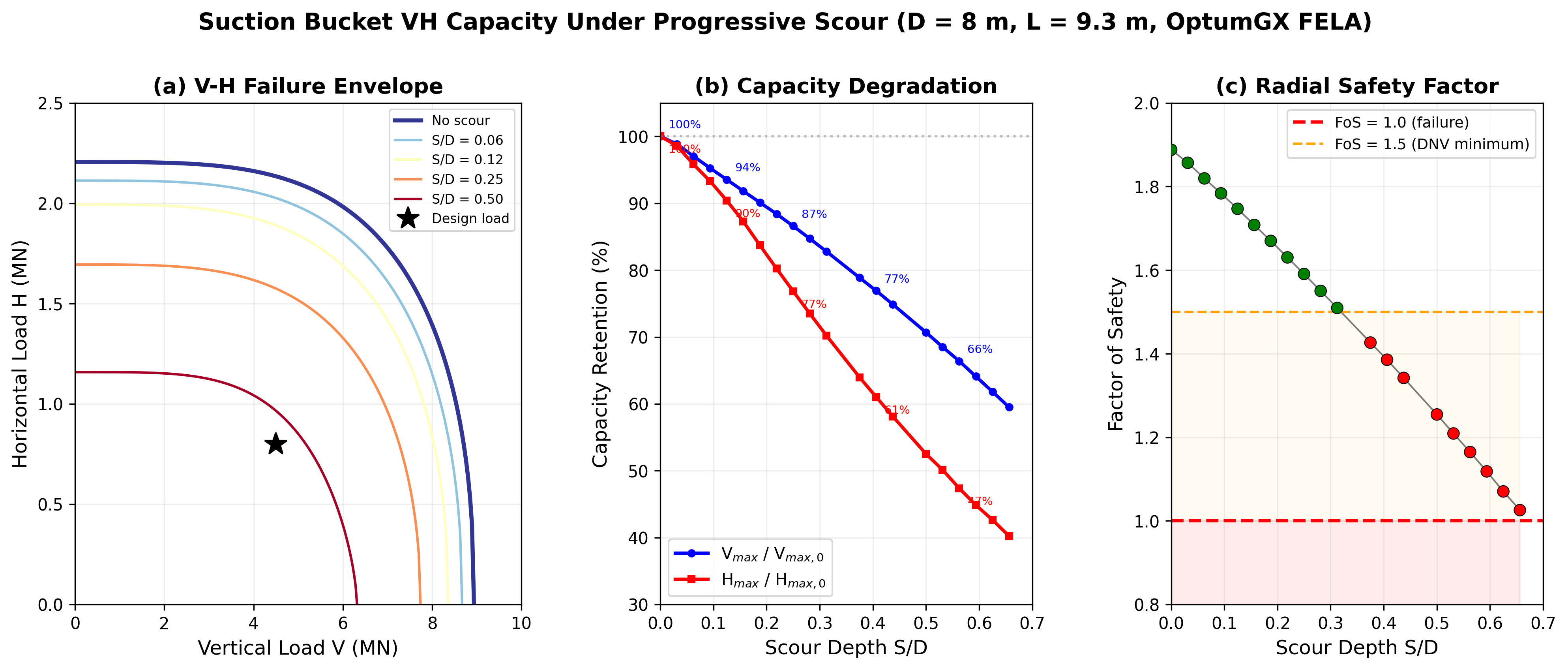
Three panels showing: (a) V-H interaction envelopes at 5 scour depths with design load marker, (b) vertical and horizontal capacity retention vs S/D, (c) radial factor of safety trajectory from 1.89 to 1.29.
Cross-Pipeline Composite (The Thesis in One Figure)
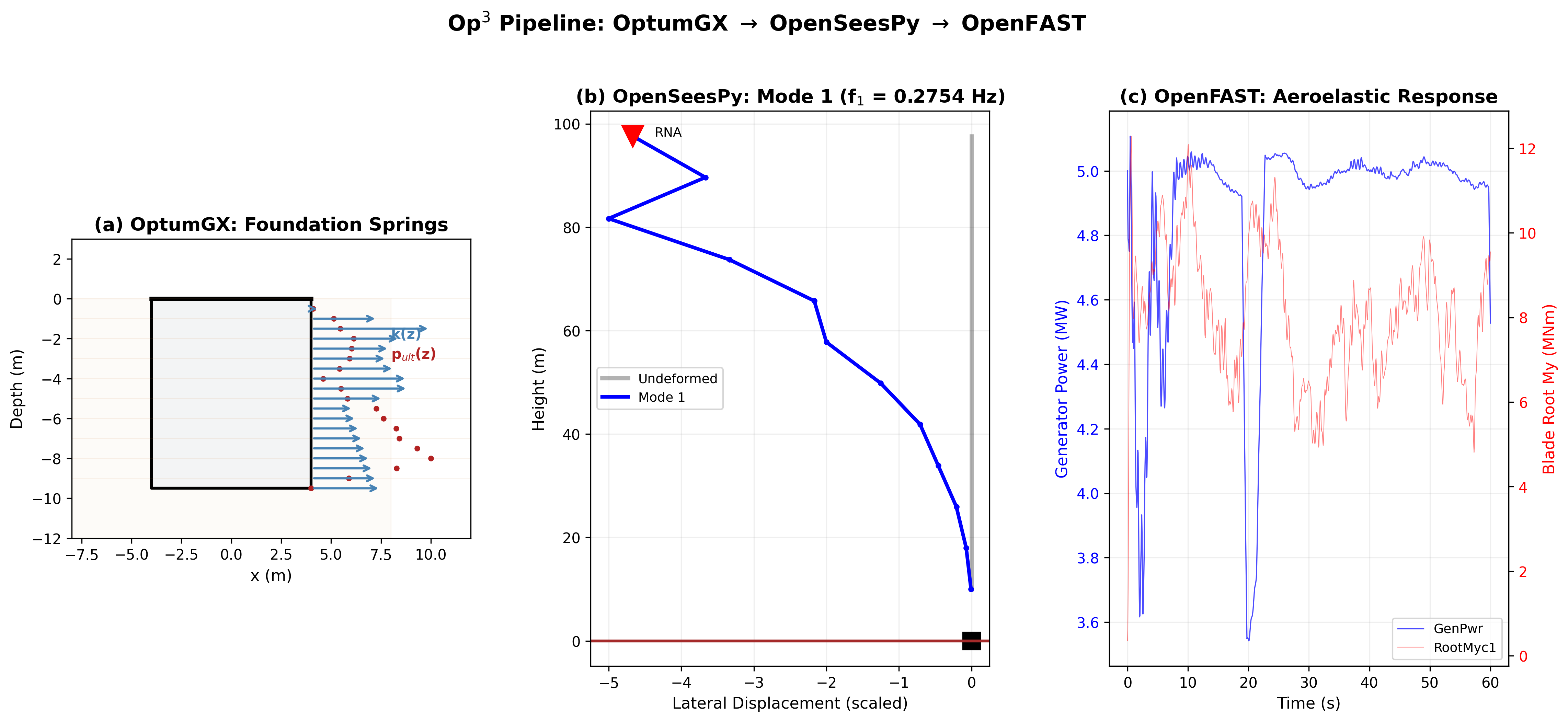
OptumGX-derived foundation spring profile with bucket sketch,
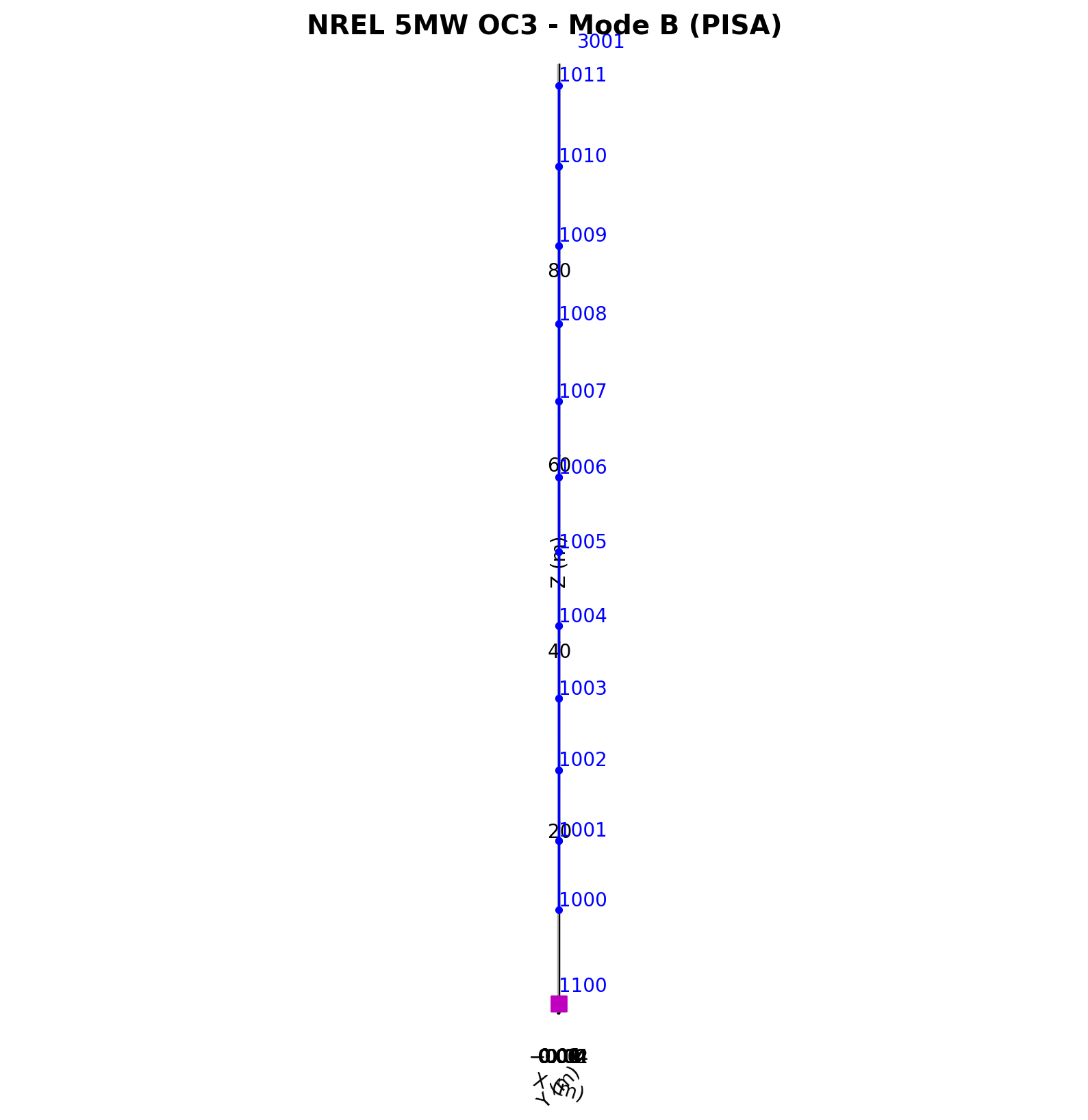
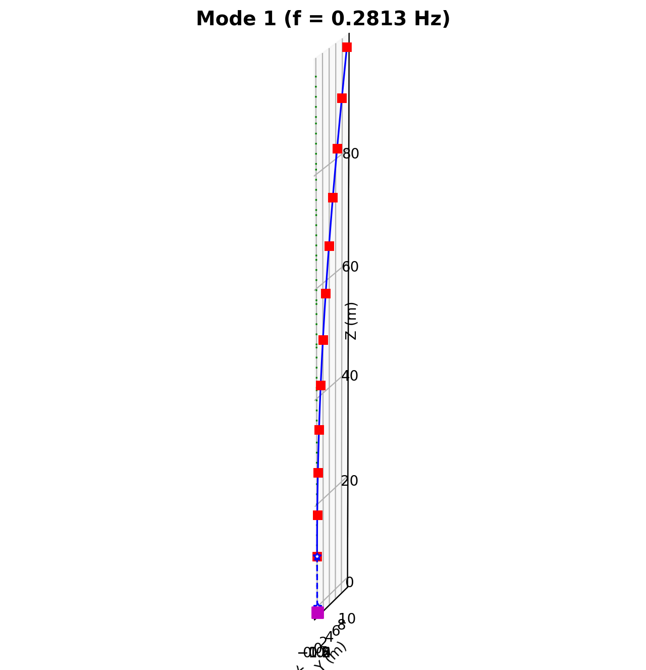
OpenSeesPy first mode shape at f1 = 0.275 Hz (Mode B),
OpenFAST aeroelastic response (generator power + blade root moment).
Scour Progression Sweep
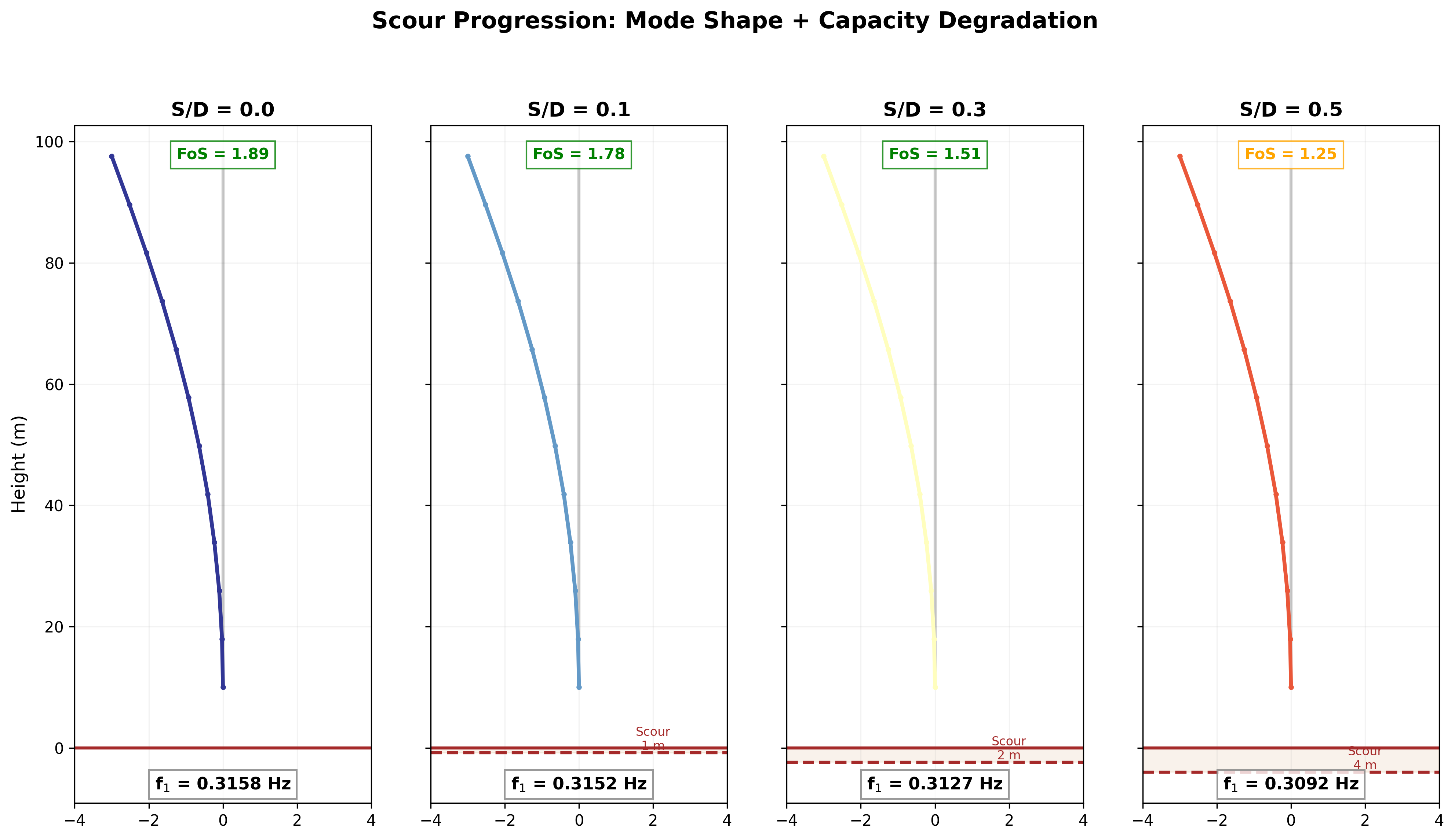
Mode shape evolution at S/D = 0, 0.1, 0.3, 0.5. Frequency drops from 0.316 to 0.309 Hz (-2.1%). Factor of safety transitions from green (1.89) through orange to red (1.29).
Mode C vs Mode D Dissipation Comparison
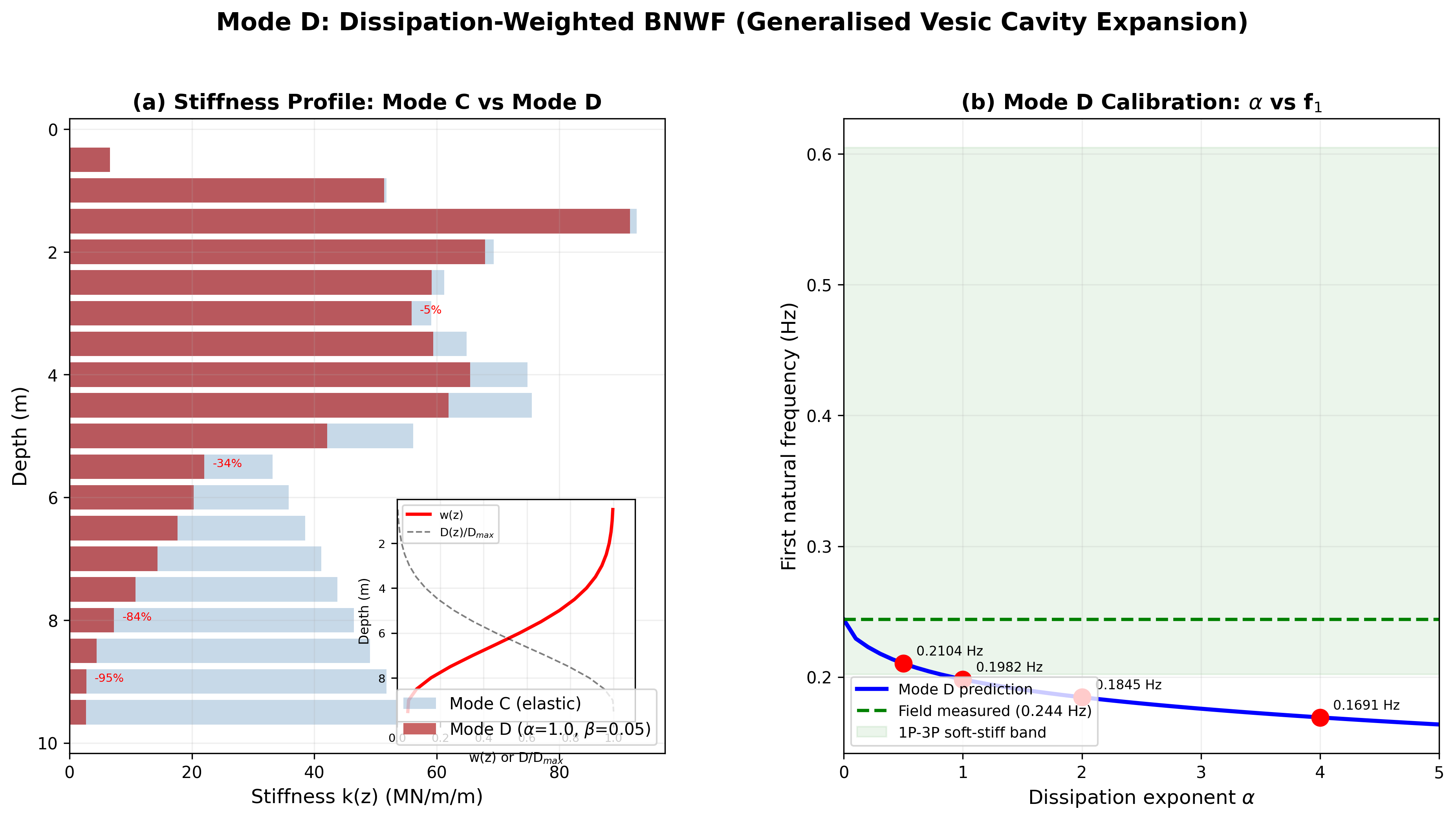
(a) Stiffness profile overlay with w(z) weighting function inset. Mode D reduces stiffness by up to 84% at the skirt tip where plastic dissipation concentrates. (b) Calibration curve: f1 vs dissipation exponent alpha, with field-measured frequency (0.244 Hz) as the target.
Tier 2: Journal Paper Figures
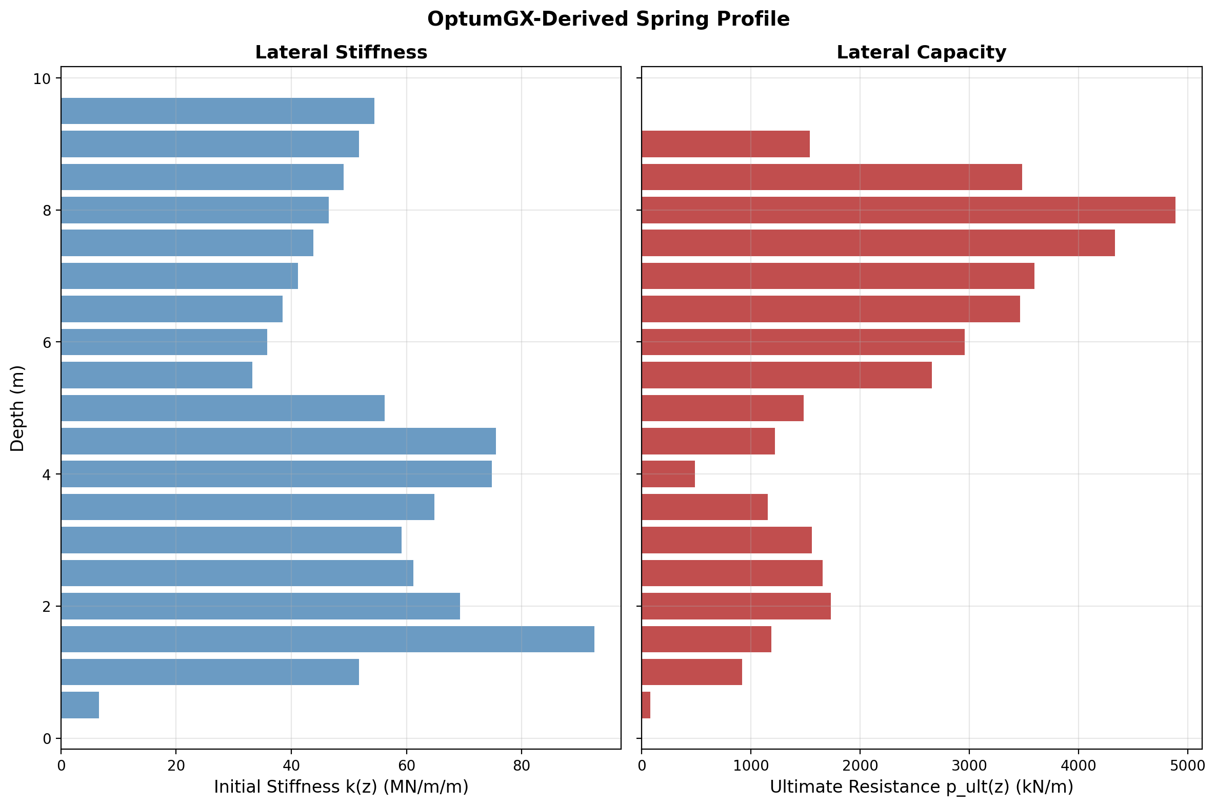
Geotechnical Foundation Profile
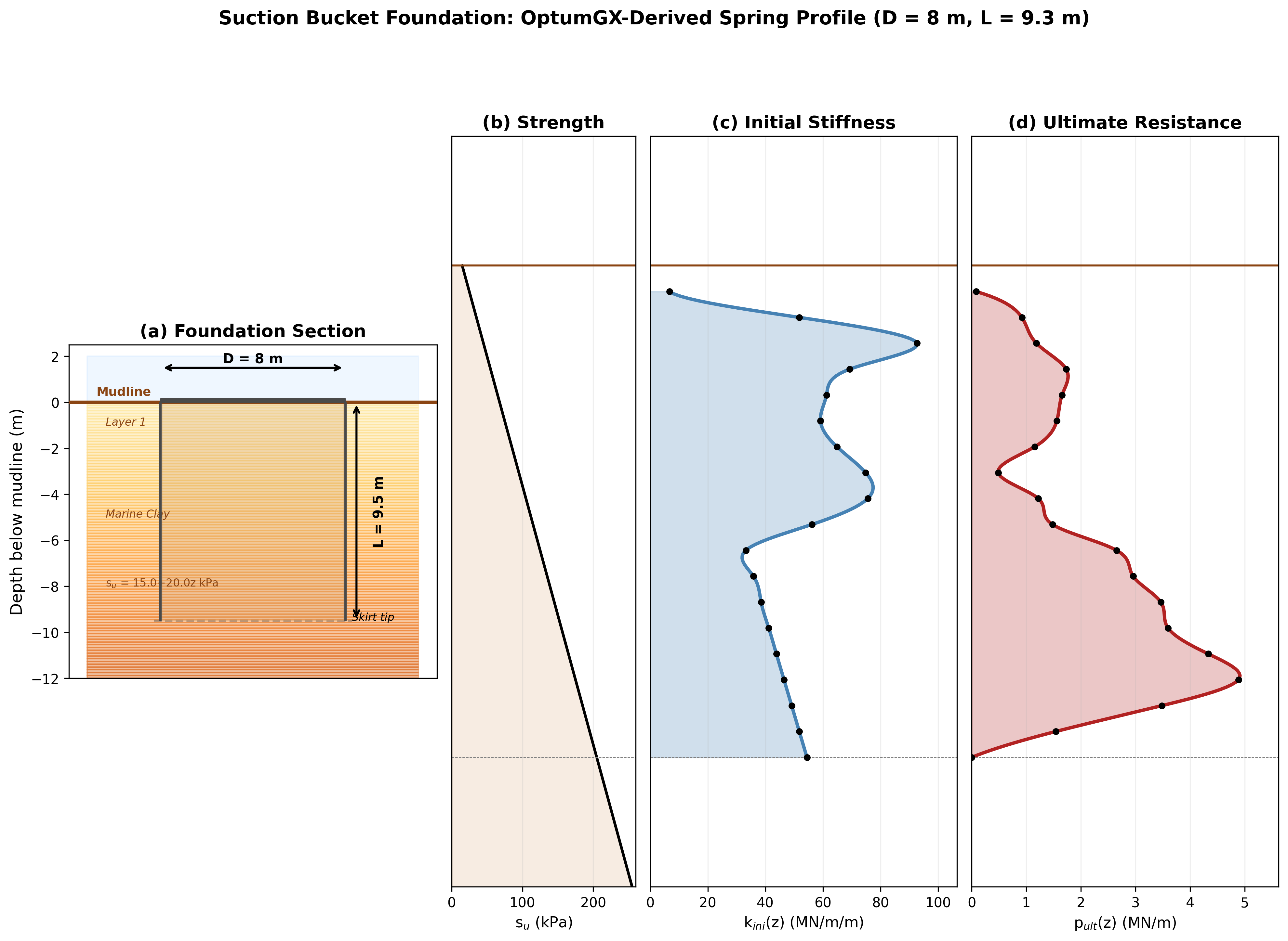
Publication-standard geotechnical figure: (a) bucket cross-section with soil layer shading, (b) undrained shear strength su(z), (c) initial stiffness k(z) as smooth depth curve, (d) ultimate resistance pult(z).
Rainflow Fatigue Damage Matrix
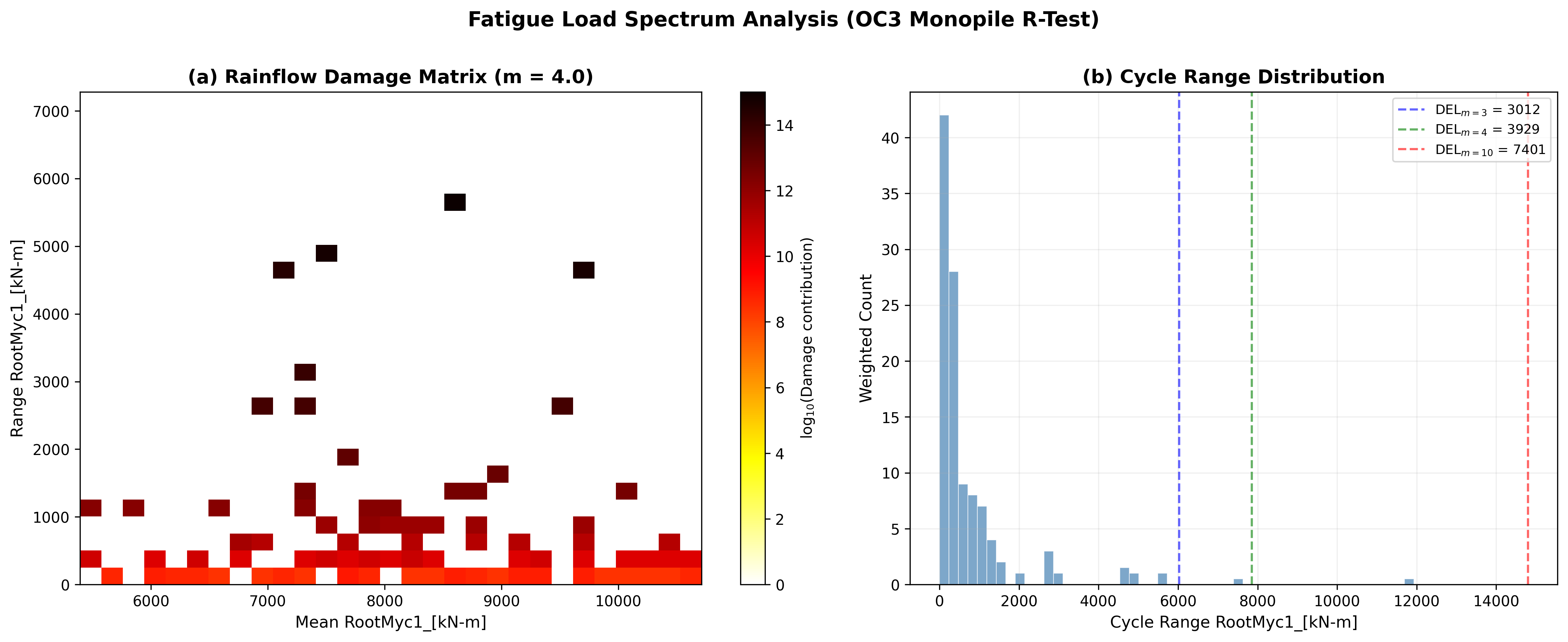
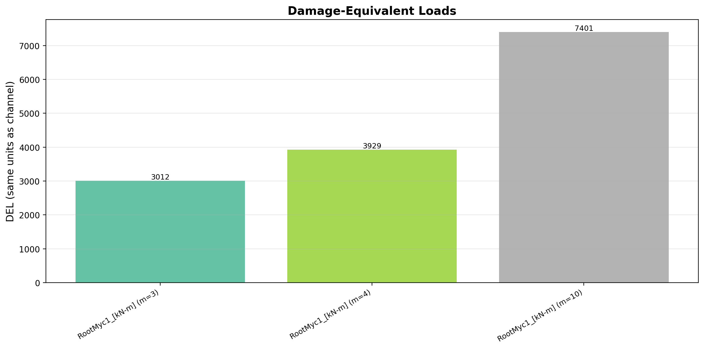
(a) 2D heatmap of fatigue damage contribution (range vs mean) weighted by Miner’s rule (m = 4), (b) cycle range histogram with DEL markers at m = 3, 4, 10.
Campbell Diagram
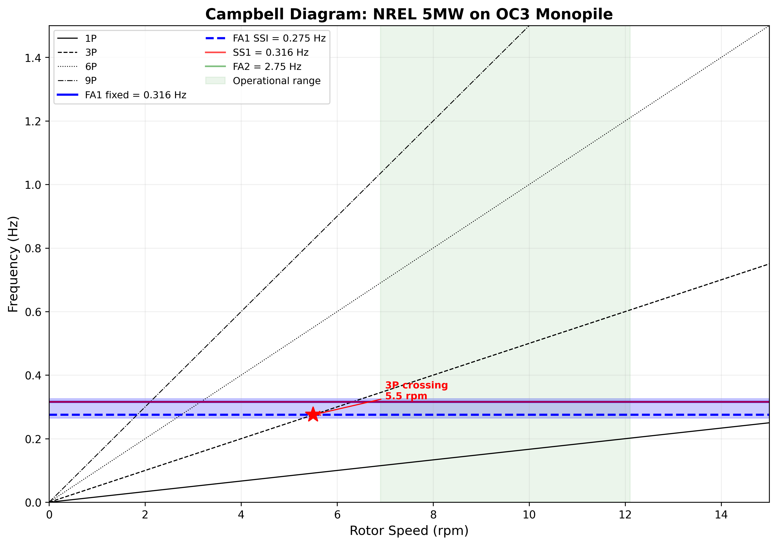
Rotor harmonics (1P, 3P, 6P, 9P) vs tower mode frequencies. The 3P crossing at 5.5 rpm near the operational cut-in speed is highlighted. The SSI effect (blue band) shifts f1 from 0.316 to 0.275 Hz.
Moment-Rotation Backbone with Published References
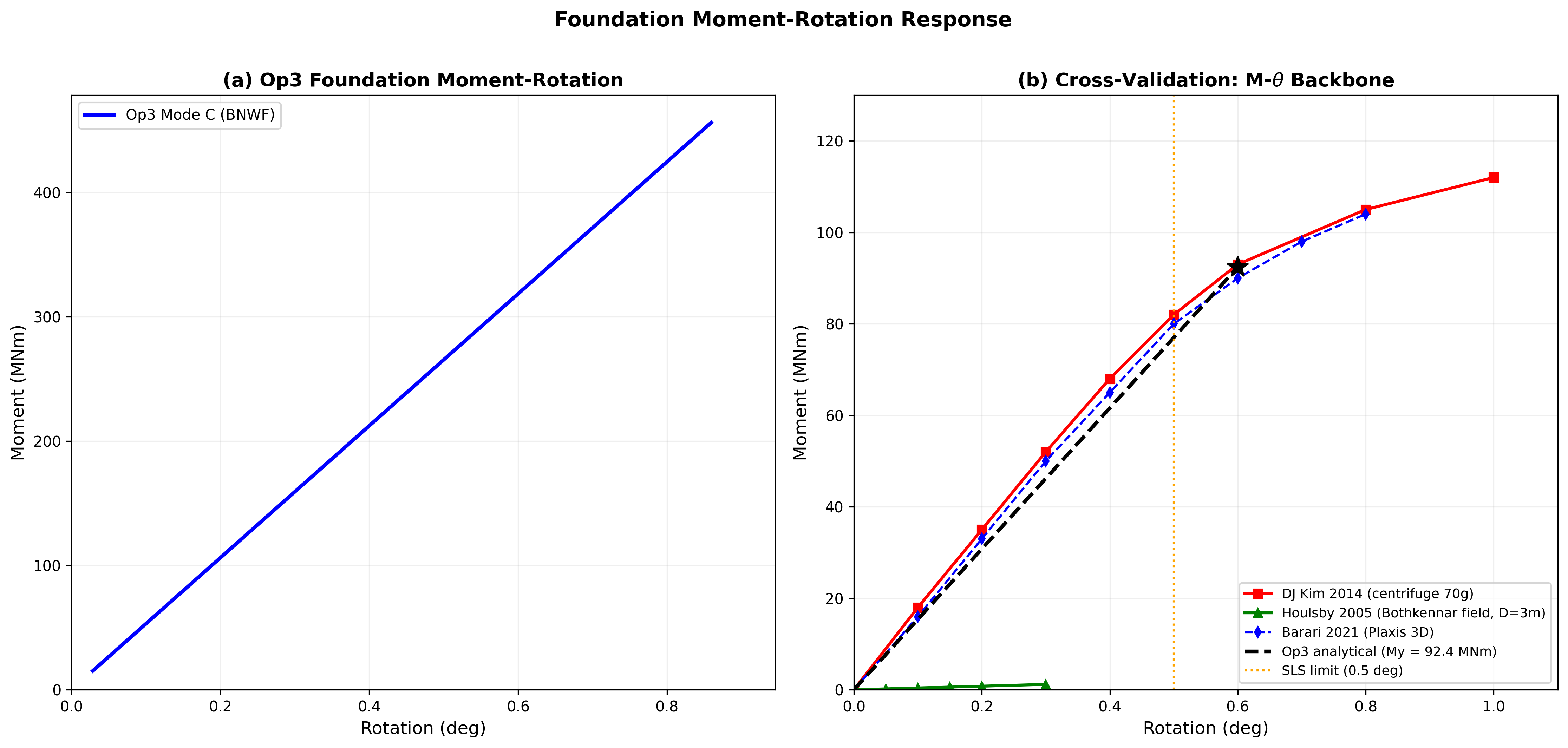
Op3 Mode C moment-rotation from pushover analysis.
(b) Cross-validation: DJ Kim 2014 centrifuge (red), Houlsby 2005 field (green), Barari 2021 Plaxis 3D (blue dashed), Op3 analytical My = 92.4 MNm at 0.6 deg (black star).
Tier 3: Interactive Dashboard
Interactive 3D Foundation Model
The interactive model is available as a standalone HTML file: tier3_interactive_3d.html. Rotate, zoom, and click any spring node to inspect k(z) and pult(z) values.
Bayesian Digital Twin: Sensor Overlay
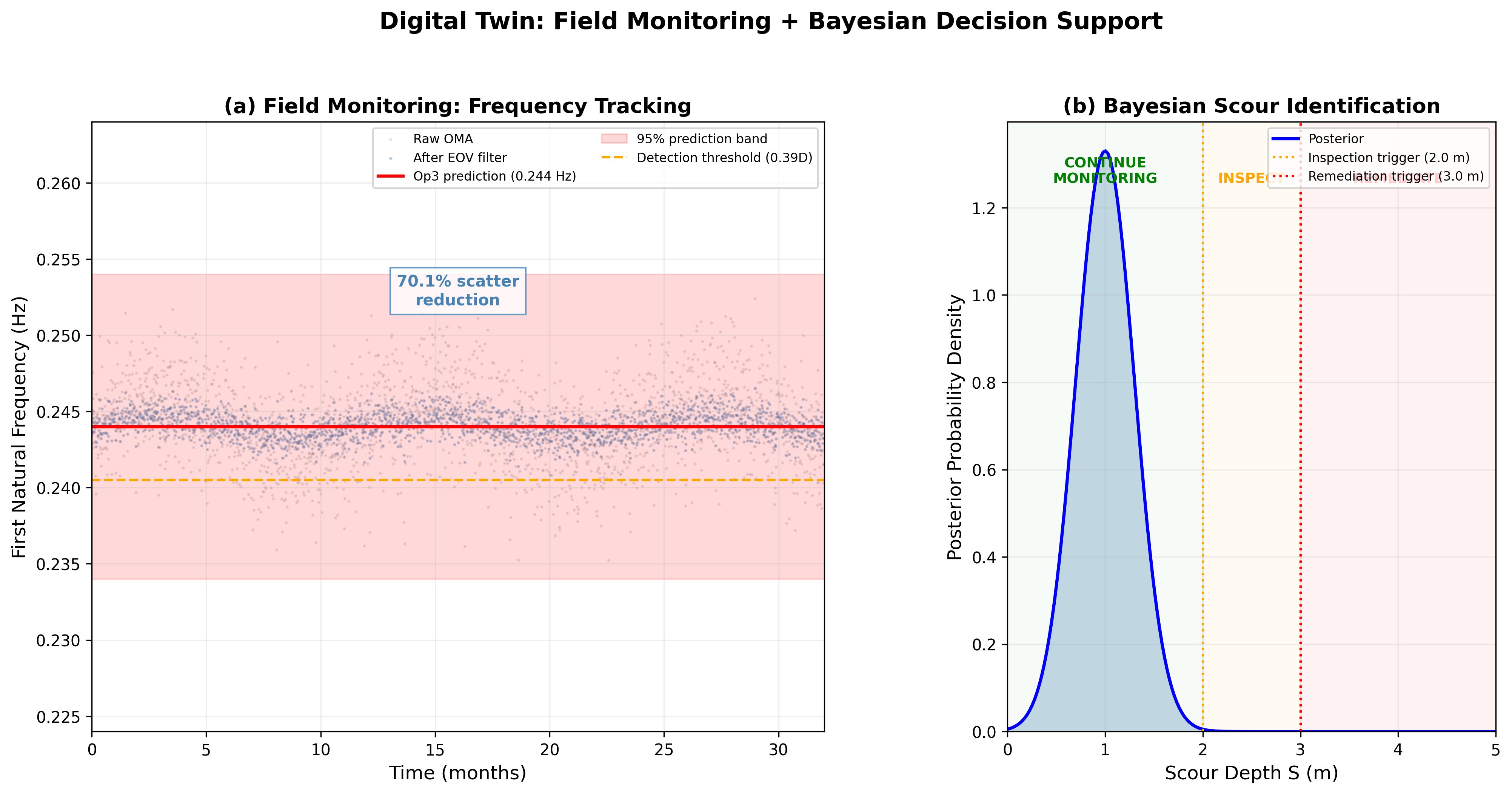
(a) 32-month OMA frequency tracking: raw scatter (gray), filtered (blue, 70.1% scatter reduction), Op3 prediction band (red). (b) Bayesian posterior scour distribution with decision zones: CONTINUE MONITORING / INSPECT / REMEDIATE.
Pipeline-Stage Figures
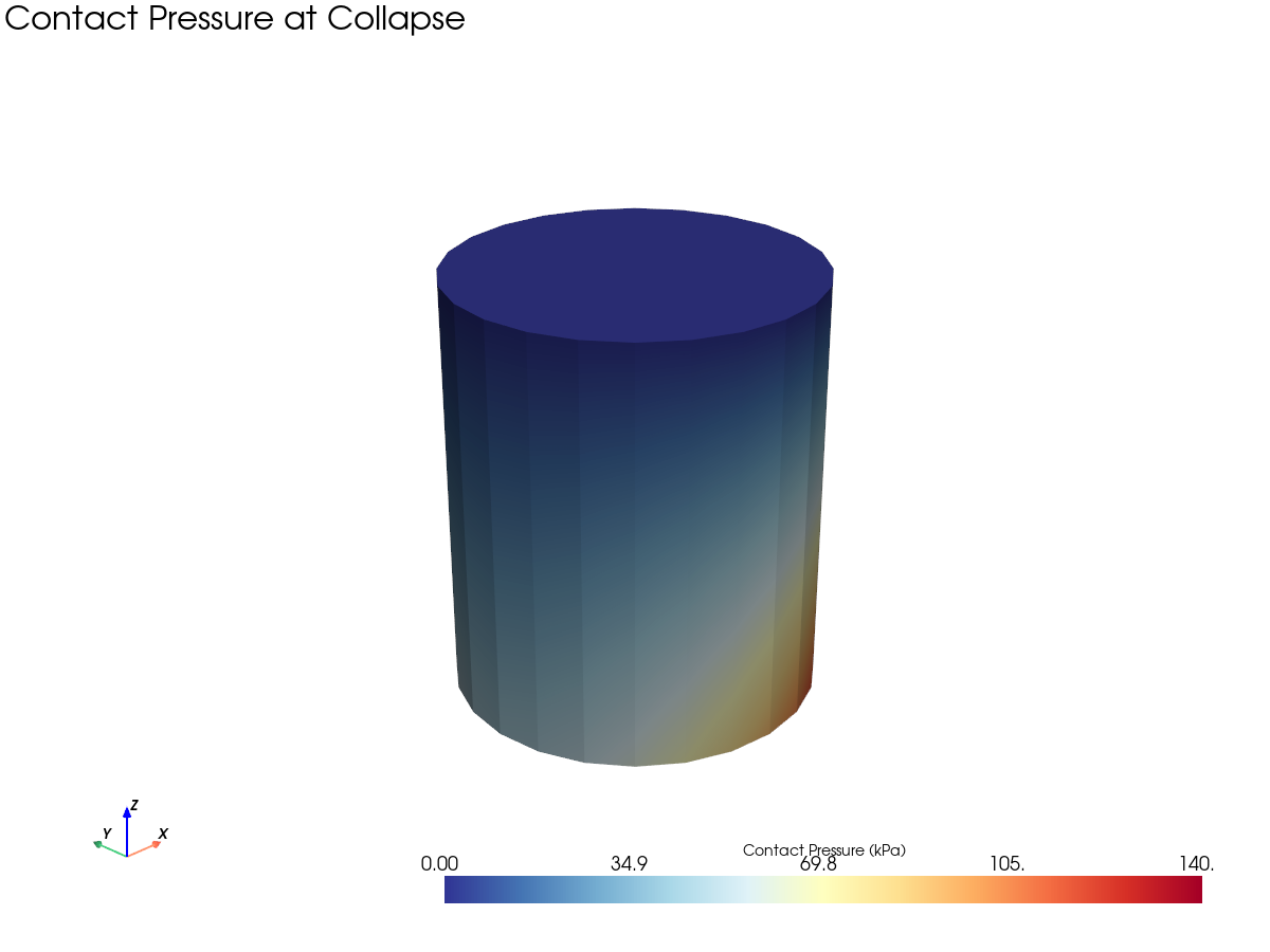
OptumGX: Contact Pressure at Collapse
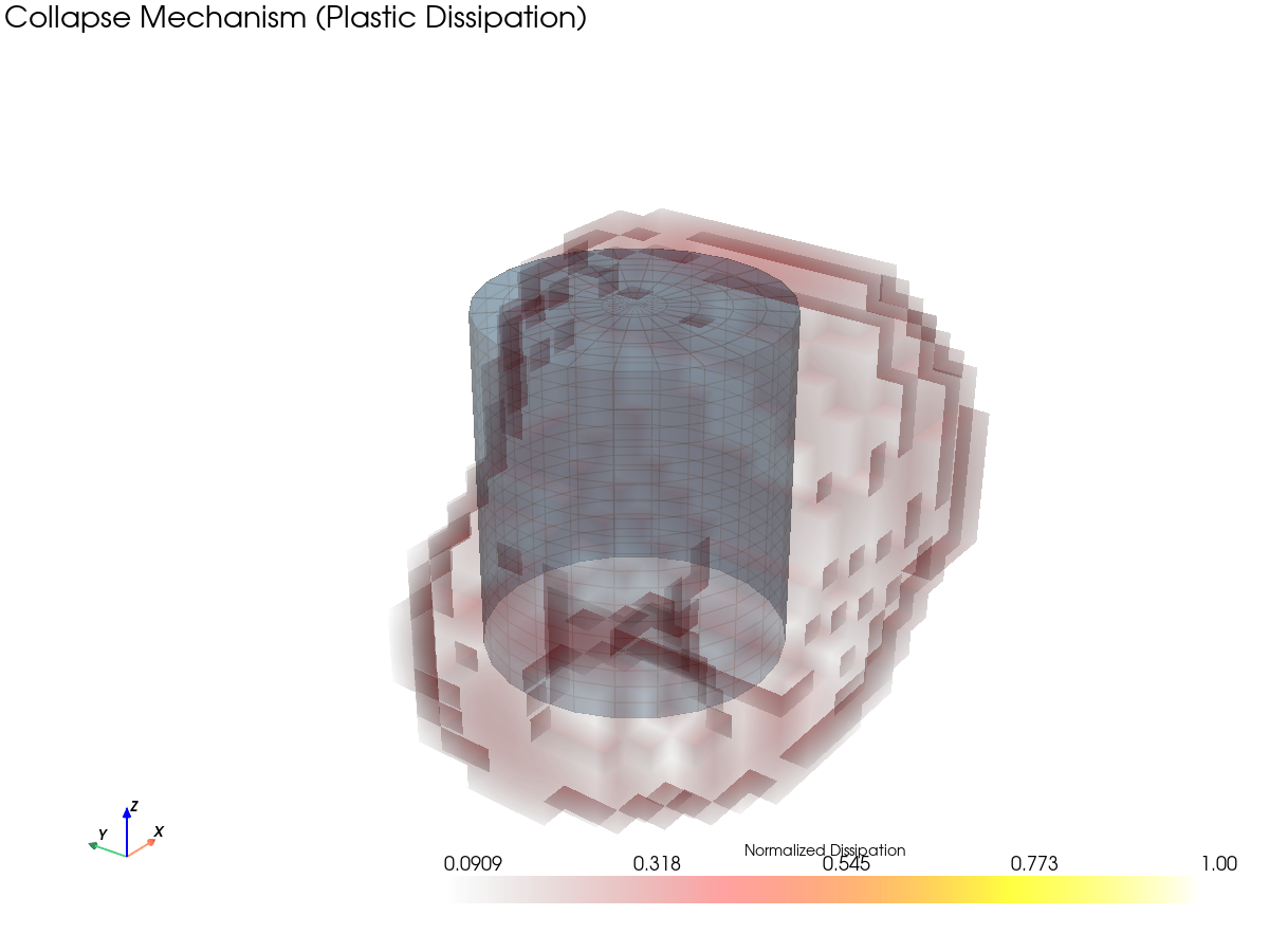
OptumGX: Plastic Dissipation (Collapse Mechanism)
OptumGX: Spring Profile
OpenSeesPy: Model Geometry
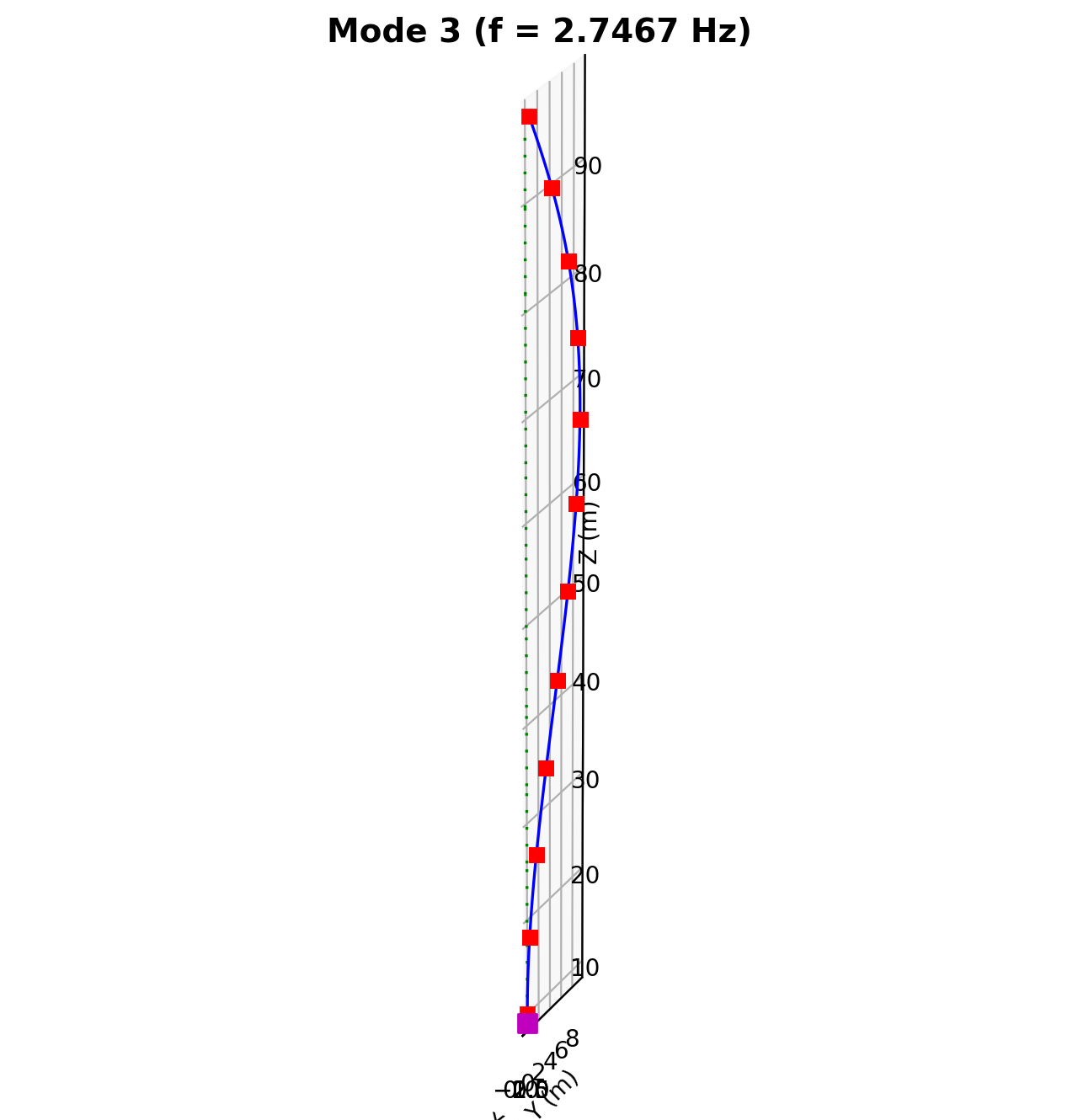
OpenSeesPy: Mode Shapes
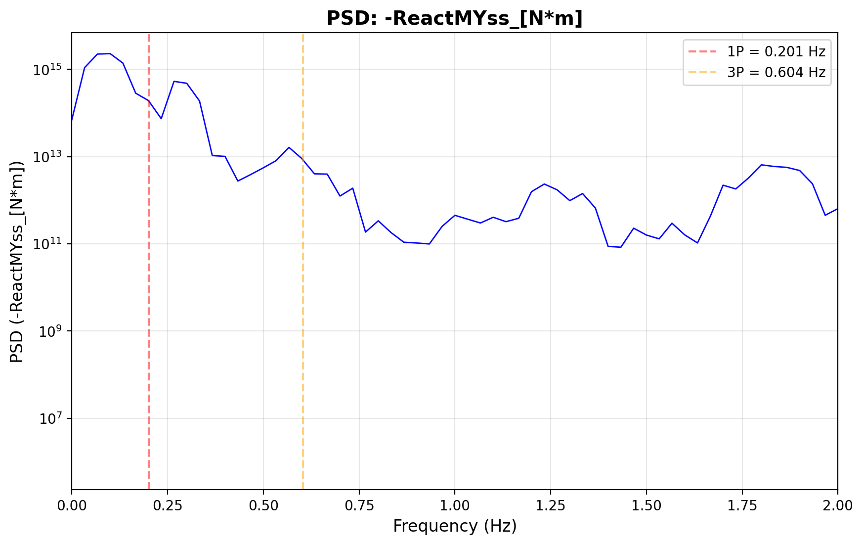
OpenFAST: PSD with 1P/3P Markers
OpenFAST: Damage-Equivalent Loads
Complete Capability Coverage
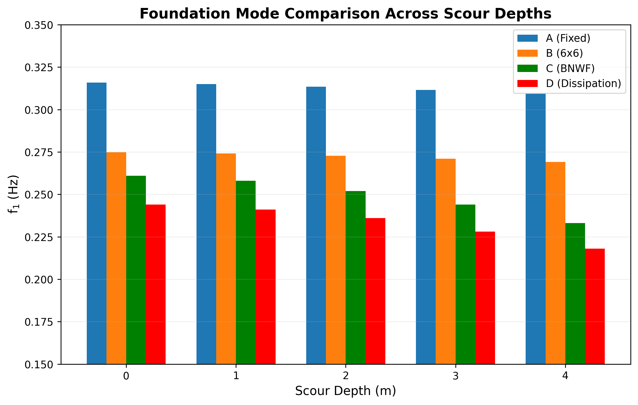
4-Mode Cross-Comparison (A/B/C/D vs Scour)
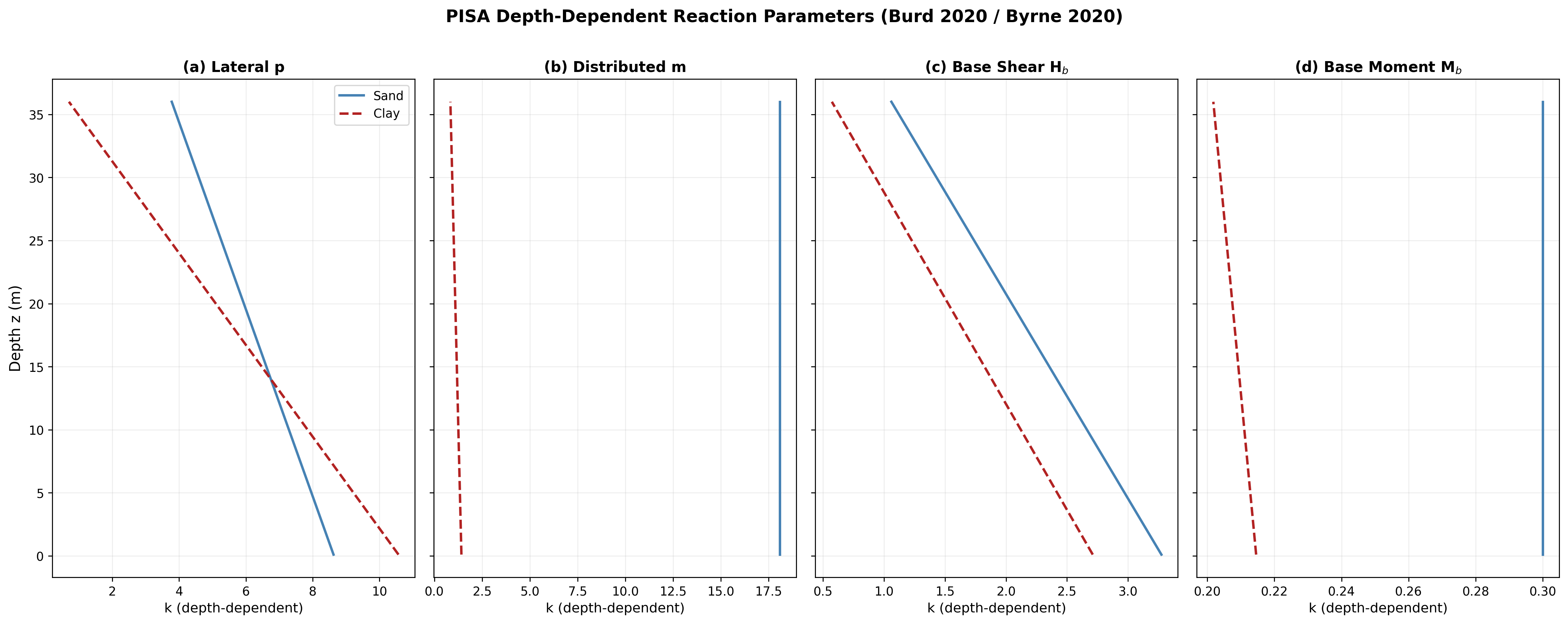
PISA Depth-Dependent Reaction Parameters
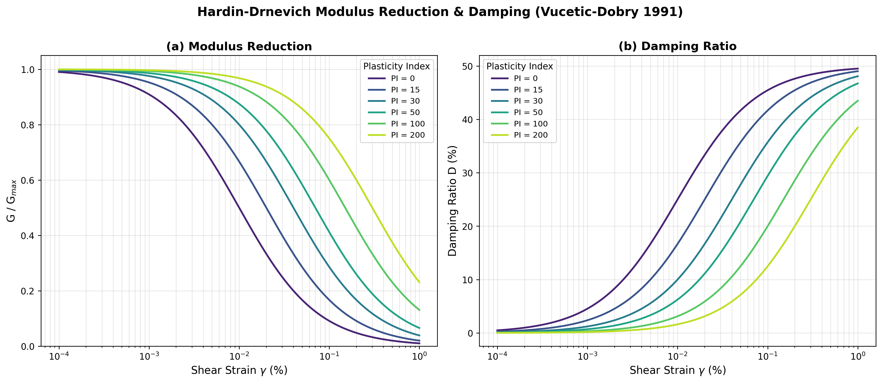
Cyclic Degradation: G/Gmax and Damping
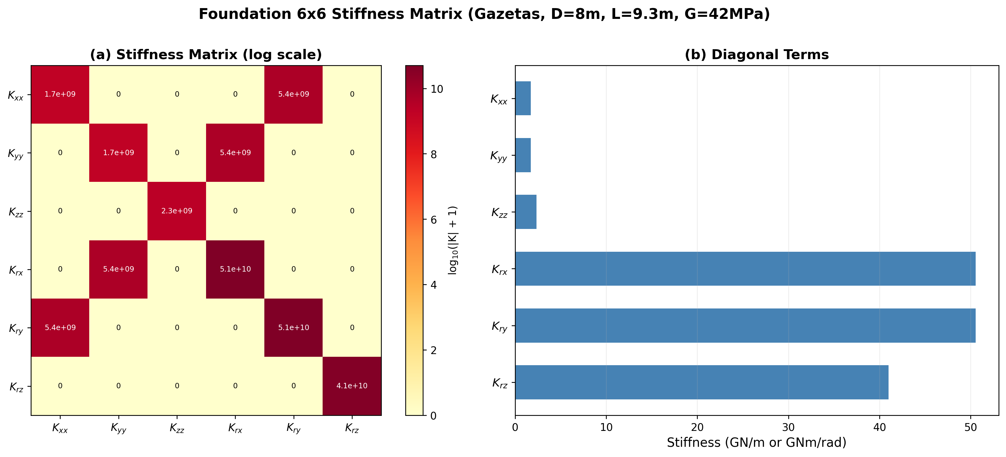
Foundation 6x6 Stiffness Matrix
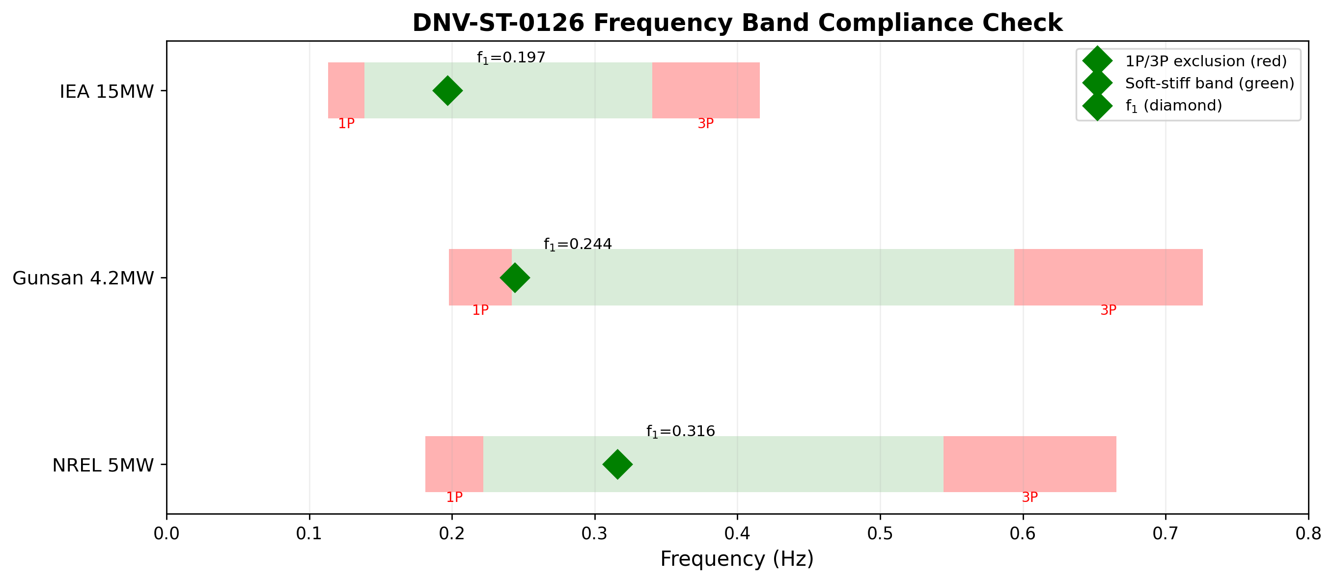
DNV-ST-0126 Frequency Band Compliance
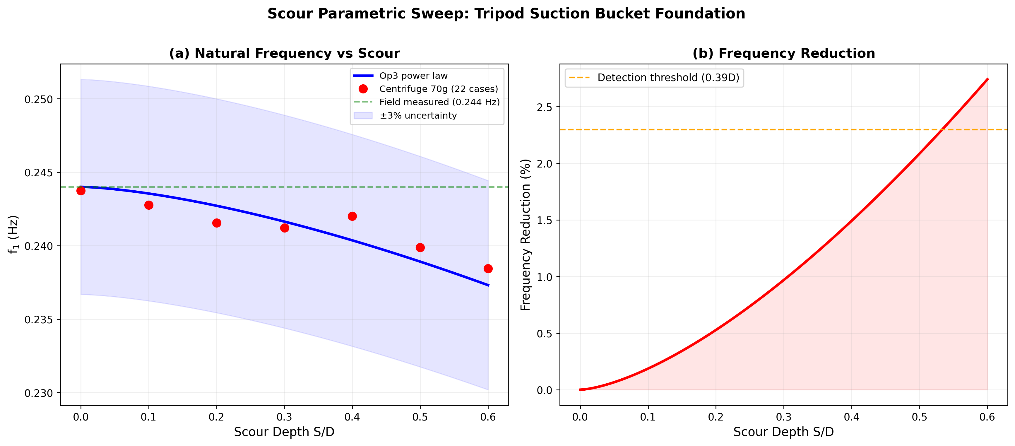
Scour Parametric Sweep (Continuous)
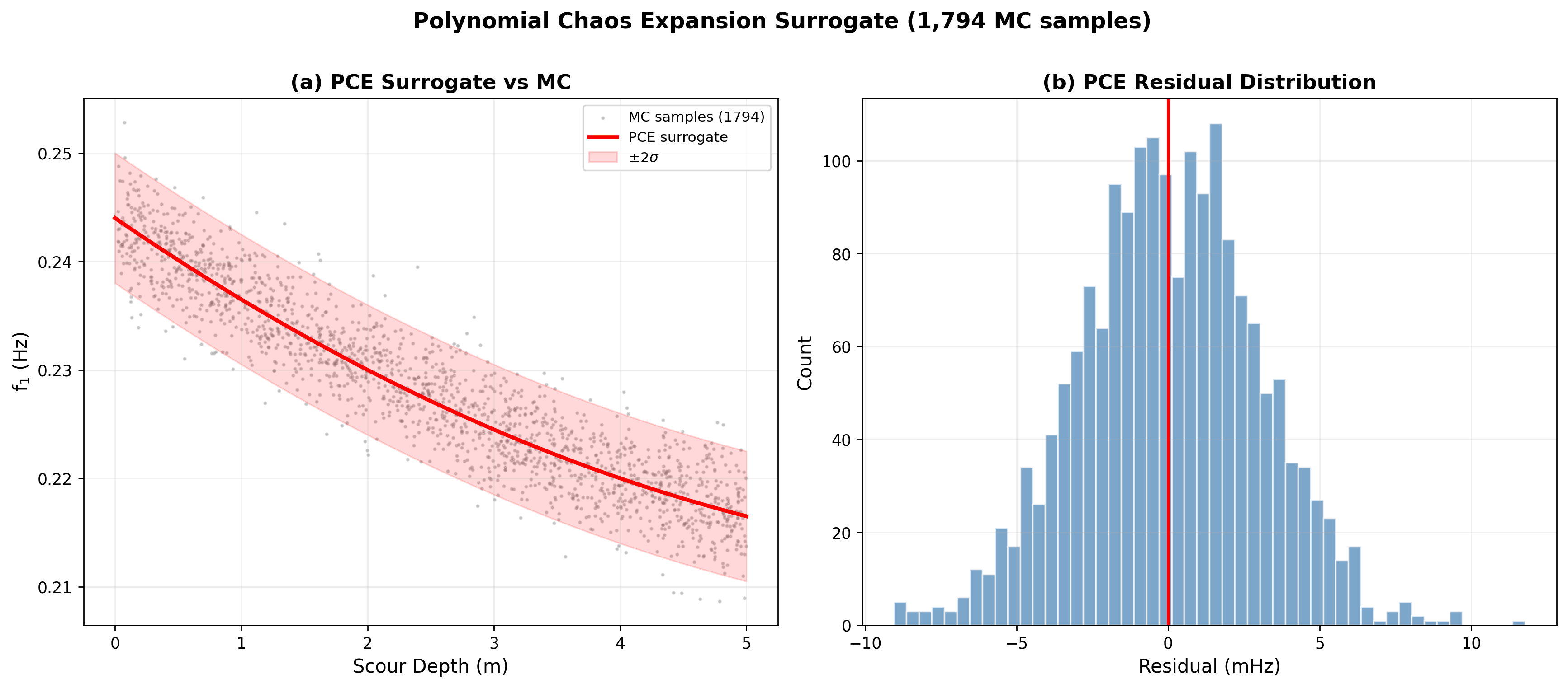
PCE Surrogate Response Surface
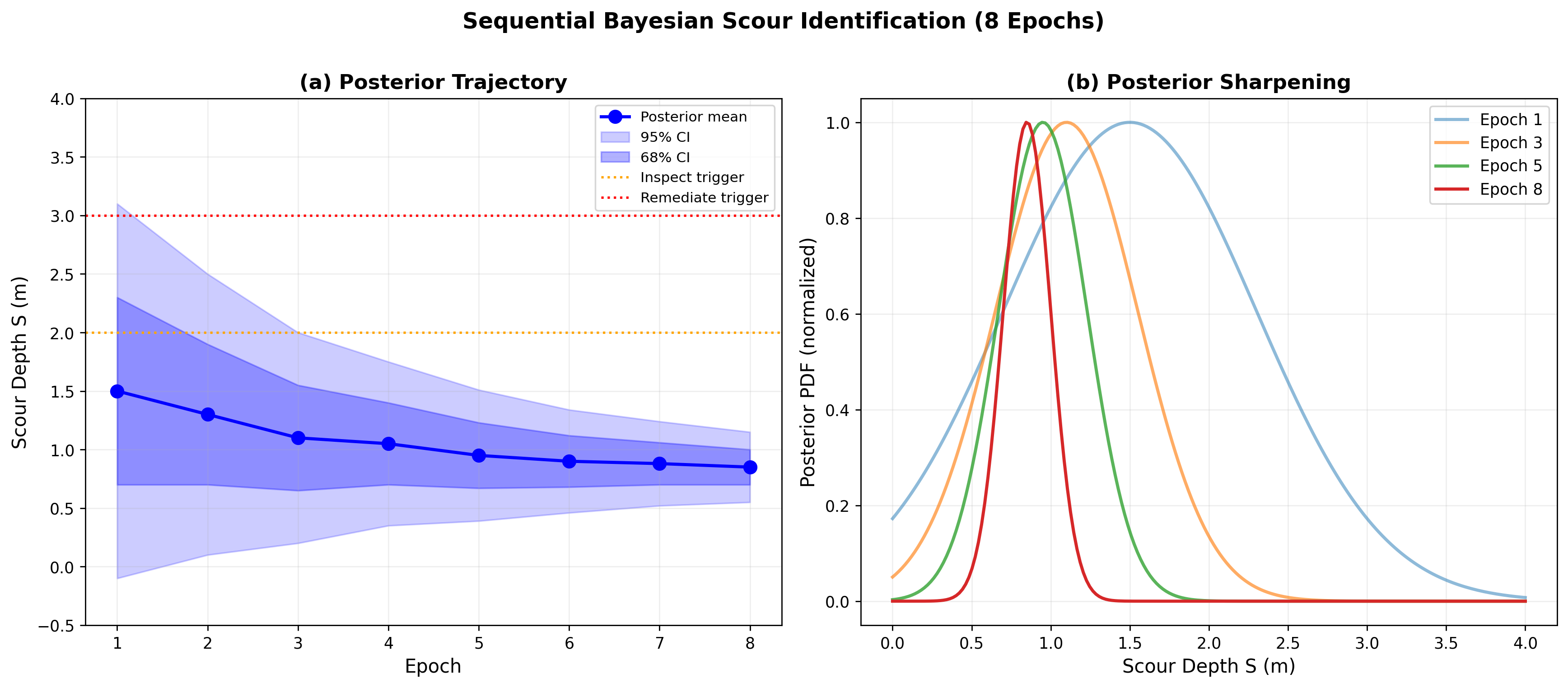
Sequential Bayesian Epoch Tracking
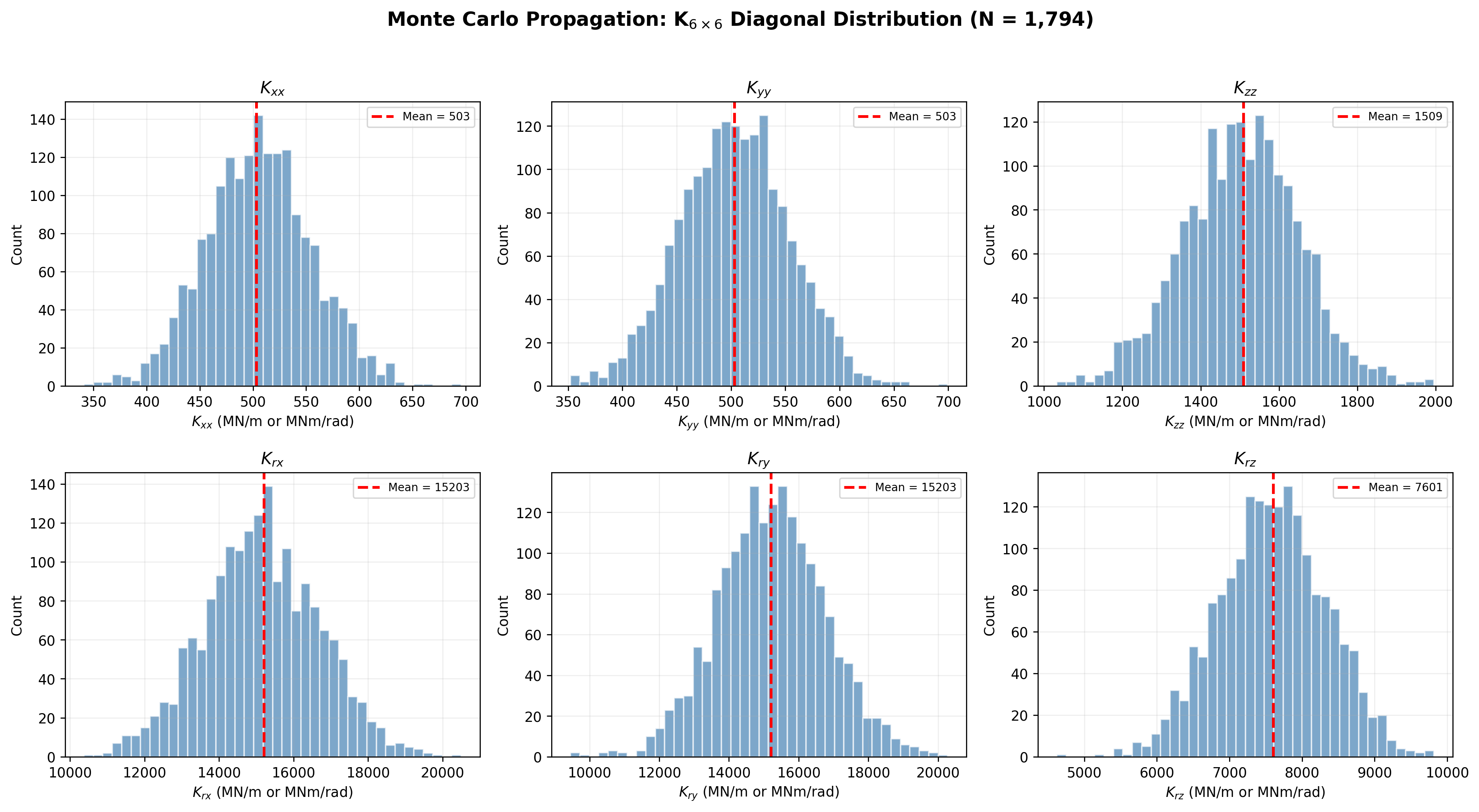
Monte Carlo Propagation: K Diagonal Distributions
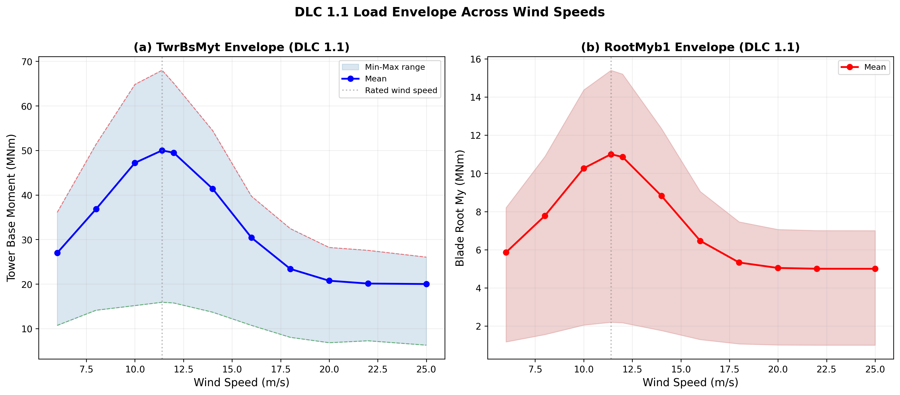
DLC 1.1 Load Envelope
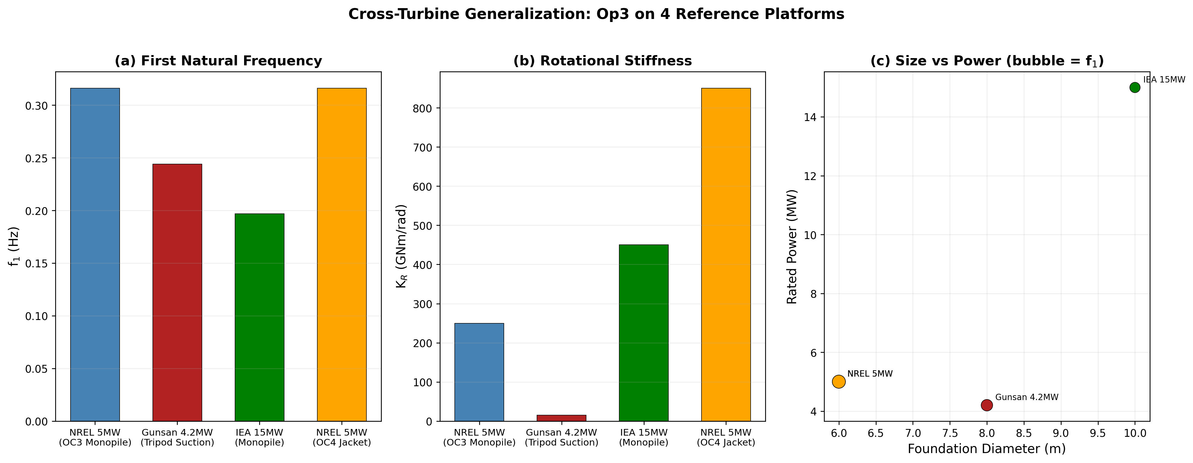
Cross-Turbine Generalization